V Measure: A Conditional Entropy Based External Cluster Evaluation Measure

V-Measure: A conditional entropy-based external cluster evaluation

measure

Andrew Rosenberg and Julia Hirschberg

Department of Computer Science Columbia University New York, NY 10027

{amaxwell,julia}@cs.columbia.edu

Abstract

We present V-measure, an external entropy-based cluster evaluation measure. V-measure provides an elegant solution to many problems that affect previously de-fined cluster evaluation measures includ-ing 1) dependence on clusterinclud-ing algorithm or data set, 2) the “problem of matching”, where the clustering of only a portion of data points are evaluated and 3) accurate evalu-ation and combinevalu-ation of two desirable as-pects of clustering, homogeneity and com-pleteness. We compare V-measure to a num-ber of popular cluster evaluation measures and demonstrate that it satisfies several de-sirable properties of clustering solutions, us-ing simulated clusterus-ing results. Finally, we use V-measure to evaluate two clustering tasks: document clustering and pitch accent type clustering.

1 Introduction

Clustering techniques have been used successfully for many natural language processing tasks, such as document clustering (Willett, 1988; Zamir and Etzioni, 1998; Cutting et al., 1992; Vempala and Wang, 2005), word sense disambiguation (Shin and Choi, 2004), semantic role labeling (Baldewein et al., 2004), pitch accent type disambiguation (Levow, 2006). They are particularly appealing for tasks in which there is an abundance of language data available, but manual annotation of this data is very resource-intensive. Unsupervised clustering can eliminate the need for (full) manual annotation of the data into desired classes, but often at the cost of making evaluation of success more difficult.

External evaluation measures for clustering can be applied when class labels for each data point in some evaluation set can be determined a priori. The

clustering task is then to assign these data points to any number of clusters such that each cluster con-tains all and only those data points that are members of the same class Given the ground truth class la-bels, it is trivial to determine whether this perfect clustering has been achieved. However, evaluating how far from perfect an incorrect clustering solution is a more difficult task (Oakes, 1998) and proposed approaches often lack rigor (Meila, 2007).

In this paper, we describe a new entropy-based external cluster evaluation measure, V-MEASURE1, designed to address the problem of quantifying such imperfection. Like all external measures, V-measure compares a target clustering — e.g., a manually an-notated representative subset of the available data — against an automatically generated clustering to de-termine now similar the two are. We introduce two complementary concepts, completeness and homo-geneity, to capture desirable properties in clustering tasks.

In Section 2, we describe V-measure and how it is calculated in terms of homogeneity and complete-ness. We describe several popular external cluster evaluation measures and draw some comparisons to V-measure in Section 3. In Section 4, we discuss how some desirable properties for clustering are sat-isfied by V-measure vs. other measures. In Sec-tion 5, we present two applicaSec-tions of V-measure, on document clustering and on pitch accent type clus-tering.

2 V-Measure and Its Calculation

V-measure is an entropy-based measure which ex-plicitly measures how successfully the criteria of ho-mogeneity and completeness have been satisfied. V-measure is computed as the harmonic mean of dis-tinct homogeneity and completeness scores, just as

1

The ‘V’ stands for “validity”, a common term used to de-scribe the goodness of a clustering solution.

precision and recall are commonly combined into F-measure (Van Rijsbergen, 1979). As F-measure scores can be weighted, V-measure can be weighted to favor the contributions of homogeneity or com-pleteness.

For the purposes of the following discussion, as-sume a data set comprising N data points, and two partitions of these: a set of classes, C = {ci|i =

1, . . . , n}and a set of clusters,K ={ki|1, . . . , m}. LetAbe the contingency table produced by the clus-tering algorithm representing the clusclus-tering solution, such thatA={aij}whereaij is the number of data points that are members of classci and elements of clusterkj.

To discuss cluster evaluation measures we intro-duce two criteria for a clustering solution: homo-geneity and completeness. A clustering result sat-isfies homogeneity if all of its clusters contain only data points which are members of a single class. A clustering result satisfies completeness if all the data points that are members of a given class are elements of the same cluster. The homogenity and complete-ness of a clustering solution run roughly in opposi-tion: Increasing the homogeneity of a clustering so-lution often results in decreasing its completeness. Consider, two degenerate clustering solutions. In one, assigning every datapoint into a single cluster, guarantees perfect completeness — all of the data points that are members of the same class are triv-ially elements of the same cluster. However, this cluster is as unhomogeneous as possible, since all classes are included in this single cluster. In an-other solution, assigning each data point to a dis-tinct cluster guarantees perfect homogeneity — each cluster trivially contains only members of a single class. However, in terms of completeness, this so-lution scores very poorly, unless indeed each class contains only a single member. We define the dis-tance from a perfect clustering is measured as the weighted harmonic mean of measures of homogene-ity and completeness.

Homogeneity:

In order to satisfy our homogeneity criteria, a clustering must assign only those datapoints that are members of a single class to a single cluster. That is, the class distribution within each cluster should be skewed to a single class, that is, zero entropy. We de-termine how close a given clustering is to this ideal

by examining the conditional entropy of the class distribution given the proposed clustering. In the perfectly homogeneous case, this value, H(C|K), is 0. However, in an imperfect situation, the size of this value, in bits, is dependent on the size of the dataset and the distribution of class sizes. There-fore, instead of taking the raw conditional entropy, we normalize this value by the maximum reduction in entropy the clustering information could provide, specifically,H(C).

Note thatH(C|K)is maximal (and equalsH(C)) when the clustering provides no new information — the class distribution within each cluster is equal to the overall class distribiution. H(C|K) is 0 when each cluster contains only members of a single class, a perfectly homogenous clustering. In the degen-erate case whereH(C) = 0, when there is only a single class, we define homogeneity to be 1. For a perfectly homogenous solution, this normalization,

H(C|K)

H(C) , equals 0. Thus, to adhere to the convention

of 1 being desirable and 0 undesirable, we define ho-mogeneity as:

h=

(

1 ifH(C, K) = 0

1− H_H(C_(C|K₎) else (1)

where

H(C|K) = − |K| X

k=1

|C| X

c=1

ack

N log ack

P|C|

c=1ack

H(C) = − |C| X

c=1

P|K|

k=1ack

n log P|K|

k=1ack

n

Completeness:

Completeness is symmetrical to homogeneity. In order to satisfy the completeness criteria, a cluster-ing must assign all of those datapoints that are mem-bers of a single class to a single cluster. To eval-uate completeness, we examine the distribution of cluster assignments within each class. In a perfectly complete clustering solution, each of these distribu-tions will be completely skewed to a single cluster. We can evaluate this degree of skew by calculat-ing the conditional entropy of the proposed cluster distribution given the class of the component dat-apoints, H(K|C). In the perfectly complete case,

each class is represented by every cluster with a dis-tribution equal to the disdis-tribution of cluster sizes,

H(K|C)is maximal and equals H(K). Finally, in the degenerate case where H(K) = 0, when there is a single cluster, we define completeness to be 1. Therefore, symmetric to the calculation above, we define completeness as:

c=

(

1 ifH(K, C) = 0

1−H_H(K_(K|C₎) else (2)

where

H(K|C) = − |C| X

c=1

|K| X

k=1

ack

N log ack

P|K|

k=1ack

H(K) = − |K| X

k=1

P|C|

c=1ack

n log P|C|

c=1ack

n

Based upon these calculations of homogeneity and completeness, we then calculate a clustering solution’s V-measure by computing the weighted harmonic mean of homogeneity and completeness,

Vβ = (1+_(β∗β_h)₎₊∗h_c∗c. Similarly to the familiar F-measure, if β is greater than 1 completeness is weighted more strongly in the calculation, ifβis less than 1, homogeneity is weighted more strongly.

Notice that the computations of homogeneity, completeness and V-measure are completely inde-pendent of the number of classes, the number of clusters, the size of the data set and the clustering al-gorithm used. Thus these measures can be applied to and compared across any clustering solution, regard-less of the number of data points (n-invariance), the number of classes or the number of clusters. More-over, by calculating homogeneity and completeness separately, a more precise evaluation of the perfor-mance of the clustering can be obtained.

3 Existing Evaluation Measures

Clustering algorithms divide an input data set into a number of partitions, or clusters. For tasks where some target partition can be defined for testing pur-poses, we define a “clustering solution” as a map-ping from each data point to its cluster assignments in both the target and hypothesized clustering. In the context of this discussion, we will refer to the target partitions, or clusters, asCLASSES, referring only to hypothesized clusters asCLUSTERS.

Two commonly used external measures for as-sessing clustering success areP urityandEntropy

(Zhao and Karypis, 2001), defined as,

P urity=Pk

r=1n1maxi(nir)

Entropy=Pk

r=1 nrn(−log1q

Pq

i=1

ni r nr log

ni r nr) where q is the number of classes, k the number of clusters, nr is the size of clusterr, andnir is the number of data points in classiclustered in cluster

r.

Both these approaches represent plausable ways to evaluate the homogeneity of a clustering solution. However, our completeness criterion is not mea-sured at all. That is, they do not address the ques-tion of whether all members of a given class are in-cluded in a single cluster. Therefore theP urityand

Entropymeasures are likely to improve (increased

P urity, decreased Entropy) monotonically with the number of clusters in the result, up to a degen-erate maximum where there are as many clusters as data points. However, clustering solutions rated high by either measure may still be far from ideal.

Another frequently used external clustering eval-uation measure is commonly refered to as “cluster-ing accuracy”. The calculation of this accuracy is inspired by the information retrieval metric of F-Measure (Van Rijsbergen, 1979). The formula for this clustering F-measure as described in (Fung et al., 2003) is shown in Figure 3.

LetN be the number of data points,C the set of classes,K

the set of clusters andnijbe the number of members of class

ci∈Cthat are elements of clusterkj∈K.

F(C, K) = X c_i∈C

|ci|

N kmaxj∈K{F(ci, kj)} (3)

F(ci, kj) =

2∗R(ci, kj)∗P(ci, kj)

R(ci, kj) +P(ci, kj)

R(ci, kj) =

nij |ci|

P(ci, kj) =

nij |kj|

Figure 1: Calculation of clustering F-measure

This measure has a significant advantage over

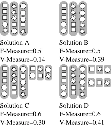
por-Solution A Solution B F-Measure=0.5 F-Measure=0.5 V-Measure=0.14 V-Measure=0.39

Solution C Solution D F-Measure=0.6 F-Measure=0.6 V-Measure=0.30 V-Measure=0.41

Figure 2: Examples of the Problem of Matching

tion of clusterjthat is a member of classi, thus mea-suring how homogenous clusterjis with respect to classi.

Like some other external cluster evaluation tech-niques (misclassification index (MI) (Zeng et al., 2002),H (Meila and Heckerman, 2001),L(Larsen and Aone, 1999), D (van Dongen, 2000), micro-averaged precision and recall (Dhillon et al., 2003)), F-measure relies on a post-processing step in which each cluster is assigned to a class. These techniques share certain problems. First, they calculate the goodness not only of the given clustering solution, but also of the cluster-class matching. Therefore, in order for the goodness of two clustering solutions to be compared using one these measures, an identical post-processing algorithm must be used. This prob-lem can be trivially addressed by fixing the class-cluster matching function and including it in the def-inition of the measure as inH. However, a second and more critical problem is the “problem of match-ing” (Meila, 2007). In calculating the similarity be-tween a hypothesized clustering and a ‘true’ cluster-ing, these measures only consider the contributions from those clusters that are matched to a target class. This is a major problem, as two significantly differ-ent clusterings can result in iddiffer-entical scores.

In figure 2, we present some illustrative examples of the problem of matching. For the purposes of this discussion we will be using F-Measure as the mea-sure to describe the problem of matching, however,

these problems affect any measure which requires a mapping from clusters to classes for evaluation.

In the figures, the shaded regions representCLUS -TERS, the shapes represent CLASSES. In a perfect clustering, each shaded region would contain all and only the same shapes. The problem of matching can manifest itself either by not evaluating the en-tire membership of a cluster, or by not evaluating every cluster. The former situation is presented in the figures A and B in figure 2. The F-Measure of both of these clustering solutions in 0.6. (The preci-sion and recall for each class is 3₅.) That is, for each class, the best or “matched” cluster contains 3 of 5 elements of the class (Recall) and 3 of 5 elements of the cluster are members of the class (Precision). The make up of the clusters beyond the majority class is not evaluated by F-Measure. Solution B is a better clustering solution than solution A, in terms of both homogeneity (crudely, “each cluster contains fewer2 classes”) and completeness (“each class is contained in fewer clusters”). Indeed, the V-Measure of so-lution B (0.387) is greater than that of soso-lution A (0.135). Solutions C and D represent a case in which not every cluster is considered in the evaluation of F-Measure. In this example, the F-Measure of both solutions is 0.5 (the harmonic mean of3₅and 3₇). The small “unmatched” clusters are not measured at all in the calculation of F-Measure. Solution D is a bet-ter clusbet-tering than solution C – there are no incorrect clusterings of different classes in the small clusters. V-Measure reflects this, solution C has a V-measure of 0.30 while the V-measure of solution D is 0.41.

A second class of clustering evaluation techniques is based on a combinatorial approach which exam-ines the number of pairs of data points that are tered similarly in the target and hypothesized clus-tering. That is, each pair of points can either be 1) clustered together in both clusterings (N11), 2)

clus-tered separately in both clusterings (N00), 3)

clus-tered together in the hypothesized but not the tar-get clustering (N01) or 4) clustered together in the

target but not in the hypothesized clustering (N10).

Based on these 4 values, a number of measures have been proposed, including Rand Index (Rand, 1971),

2

Adjusted Rand Index (Hubert and Arabie, 1985),Γ statistic (Hubert and Schultz, 1976), Jaccard (Mil-ligan et al., 1983), Fowlkes-Mallows (Fowlkes and Mallows, 1983) and Mirkin (Mirkin, 1996). We il-lustrate this class of measures with the calculation of Rand Index. Rand(C, K) = N11+N00

n(n−1)/2 Rand Index

can be interpreted as the probability that a pair of points is clustered similarly (together or separately) inCandK.

Meila (2007) describes a number of poten-tial problems of this class of measures posed by (Fowlkes and Mallows, 1983) and (Wallace, 1983). The most basic is that these measures tend not to vary over the interval of[0,1]. Transformations like those applied by the adjusted Rand Index and a mi-nor adjustment to the Mirkin measure (see Section 4) can address this problem. However, pair match-ing measures also suffer from distributional prob-lems. The baseline for Fowlkes-Mallows varies sig-nificantly between0.6and 0when the ratio of data points to clusters is greater than 3 — thus includ-ing nearly all real-world clusterinclud-ing problems. Simi-larly, the Adjusted Rand Index, as demonstrated us-ing Monte Carlo simulations in (Fowlkes and Mal-lows, 1983), varies from0.5to0.95. This variance in the measure’s baseline prompts Meila to ask if the assumption of linearity following normalization can be maintained. If the behavior of the measure is so unstable before normalization can users reasonably expect stable behavior following normalization?

A final class of cluster evaluation measures are based on information theory. These measures an-alyze the distribution of class and cluster member-ship in order to determine how successful a given clustering solution is or how different two parti-tions of a data set are. We have already examined one member of this class of measures, Entropy. From a coding theory perspective, Entropy is the weighted average of the code lengths of each ter. Our V-measure is a member of this class of clus-tering measures. One significant advantage that in-formation theoretic evaluation measures have is that they provide an elegant solution to the “problem of matching”. By examining the relative sizes of the classes and clusters being evaluated, these measures all evaluate the entire membership of each cluster — not just a ‘matched’ portion.

Dom’sQ0measure (Dom, 2001) uses conditional

entropy, H(C|K) to calculate the goodness of a clustering solution. That is, given the hypothesized partition, what is the number of bits necessary to represent the true clustering?

However, this term – like the P urity and

Entropymeasures – only evaluates the homogene-ity of a solution. To measure the completeness of the hypothesized clustering, Dom includes a model cost term calculated using a coding theory argument. The overall clustering quality measure presented is the sum of the costs of representing the data (H(C|K)) and the model. The motivation for this approach is an appeal to parsimony: Given identical condi-tional entropies, H(C|K), the clustering solution with the fewest clusters should be preferred. Dom also presents a normalized version of this term,Q2,

which has a range of(0,1]with greater scores being representing more preferred clusterings.

Q0(C, K) =H(C|K)+1

n |K| X

k=1 log

h(k) +|C| −1

|C| −1

where C is the target partition, K is the hypothe-sized partition andh(k)is the size of clusterk.

Q2(C, K) = 1

n

P|C|

c=1log

h(c)+|C|−1

|C|−1

Q0(C, K)

We believe that V-measure provides two significant advantages overQ0that make it a more useful

diag-nostic tool. First,Q0does not explicitly calculate the

degree of completeness of the clustering solution. The cost term captures some of this information, since a partition with fewer clusters is likely to be more complete than a clustering solution with more clusters. However, Q0 does not explicitly address

the interaction between the conditional entropy and the cost of representing the model. While this is an application of the minimum description length (MDL) principle (Rissanen, 1978; Rissanen, 1989), it does not provide an intuitive manner for assessing our two competing criteria of homogeneity and com-pleteness. That is, at what point does an increase in conditional entropy (homogeneity) justify a reduc-tion in the number of clusters (completeness).

Another information-based clustering measure is variation of information (V I) (Meila, 2007),

as a distance measure for comparing partitions (or clusterings) of the same data. It therefore does not distinguish between hypothesized and target cluster-ings. V I has a number of useful properties. First, it satisfies the metric axioms. This quality allows users to intuitively understand howV I values com-bine and relate to one another. Secondly, it is “con-vexly additive”. That is to say, if a cluster is split, the distance from the new cluster to the original is the distance induced by the split times the size of the cluster. This property guarantees that all changes to the metric are “local”: the impact of splitting or merging clusters is limited to only those clusters in-volved, and its size is relative to the size of these clusters. Third, VI is n-invariant: the number of data points in the cluster do not affect the value of the measure.V I depends on the relative sizes of the partitions ofC andK, not on the number of points in these partitions. However,V I is bounded by the maximum number of clusters inCorK,k∗_.

With-out manual modification however, k∗ = n, where each cluster contains only a single data point. Thus, while technicallyn-invariant, the possible values of

V I are heavily dependent on the number of data points being clustered. Thus, it is difficult to com-pareV I values across data sets and clustering algo-rithms without fixingk∗, asV Iwill vary over differ-ent ranges. It is a trivial modification to modifyV I

such that it varies over [0,1]. Normalizing, V I by

lognor1/2 logk∗ guarantee this range. However,

Meila (2007) raises two potential problems with this modification. The normalization should not be ap-plied if data sets of different sizes are to be com-pared — it negates then-invariance of the measure. Additionally, if two authors apply the latter normal-ization and do not use the same value fork∗_{, their}

results will not be comparable.

While V I has a number of very useful distance properties when analyzing a single data set across a number of settings, it has limited utility as a general purpose clustering evaluation metric for use across disparate clusterings of disparate data sets. Our homogeneity (h) and completeness (c) terms both range over [0,1] and are completelyn-invariant and

k∗-invariant. Furthermore, measuring each as a ra-tio of bit lengths has greater intuitive appeal than a more opportunistic normalization.

V-measure has another advantage as a clustering

evaluation measure over V I and Q0. By

evaluat-ing homogeneity and completeness in a symmetri-cal, complementary manner, the calculation of V-measure makes their relationship clearly observable. Separate analyses of homogeneity and complete-ness are not possible with any other cluster evalu-ation measure. Moreover, by using the harmonic mean to combine homogeneity and completeness, V-measure is unique in that it can also prioritize one criterion over another, depending on the clustering task and goals.

4 Comparing Evaluation Measures

Dom (2001) describes a parametric technique for generating example clustering solutions. He then proceeds to define five “desirable properties” that clustering accuracy measures should display, based on the parameters used to generate the clustering so-lution. To compare V-measure more directly to alter-native clustering measures, we evaluate V-measure and other measures against these and two additional desirable properties.

The parameters used in generating a clustering so-lution are as follows.

• |C|The number of classes

• |K|The number of clusters

• |Knoise| Number of “noise” clusters;

|Knoise|<|K|

• |Cnoise|Number of “noise” classes;|Cnoise|<

|C|

• ǫError probability;ǫ=ǫ1+ǫ2+ǫ3.

• ǫ1 The error mass within “useful” class-cluster

pairs

• ǫ2The error mass within noise clusters

• ǫ3The error mass within noise classes

The construction of a clustering solution begins with a matching of “useful” clusters to “useful” classes3. There are|Ku|=|K| − |Knoise|“useful” clusters and|Cu|=|C| − |Cnoise|“useful” classes. The claim is useful classes and clusters are matched to each other and matched pairs contain more data points than unmatched pairs. Probability mass of 1−ǫ is evenly distributed across each match. Er-ror mass ofǫ1is evenly distributed across each pair

3

of non-matching useful class/cluster pairs. Noise clusters are those that contain data points equally from each cluster. Error mass of ǫ2 is distributed

across every “noise”-cluster/ “useful”-class pair. We extend the parameterization technique described in (Dom, 2001) in with|Cnoise|and ǫ3. Noise classes

are those that contain data points equally from each cluster. Error mass ofǫ3 is distributed across every

“useful”-cluster/“noise”-class pair. An example so-lution, along with its generating parameters is given in Figure 3.

C1 C2 C3 Cnoise1

K1 12 12 2 3

K2 2 2 12 3

Knoise1 4 4 4 0

Figure 3: Sample parametric clustering solution with n = 60,|K| = 3,|Knoise| = 1,|C| =

3,|Cnoise|= 1, ǫ1=.1, ǫ2 =.2, ǫ3 =.1

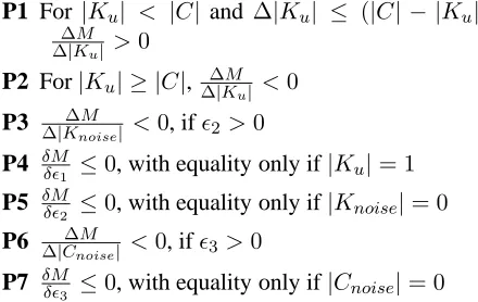
The desirable properties proposed by Dom are given as P1-P5 in Table 1. We include two addi-tional properties (P6,P7) relating the examined mea-sure value to the number of ‘noise’ classes andǫ3.

P1 For |Ku| < |C| and ∆|Ku| ≤ (|C| − |Ku|),

∆M

∆|Ku| >0

P2 For|Ku| ≥ |C|, _∆∆_|KuM_| <0

P3 _∆|Knoise∆M _| <0, ifǫ2 >0

P4 δM_δǫ1 ≤0, with equality only if|Ku|= 1

P5 δM_δǫ2 ≤0, with equality only if|Knoise|= 0

P6 _∆|Cnoise∆M _| <0, ifǫ3>0

P7 δM_δǫ3 ≤0, with equality only if|Cnoise|= 0

Table 1: Desirable Properties of a cluster evaluation measureM

To evaluate how different clustering measures sat-isfy each of these properties, we systematically var-ied each parameter, keeping|C|= 5fixed.

• |Ku|: 10 values: 2, 3,. . . , 11

• |Knoise|: 7 values: 0, 1,. . . , 6

• |Cnoise|: 7 values: 0, 1,. . . , 6

• ǫ1: 4 values: 0, 0.033, 0.066, 0.1

• ǫ2: 4 values: 0, 0.066, 0.133, 0.2

• ǫ3: 4 values: 0, 0.066, 0.133, 0.2

We evaluated the behavior of V-Measure, Rand, Mirkin, Fowlkes-Mallows, Gamma, Jaccard, VI,

Q0, F-Measure against the desirable properties

P1-P74. Based on the described systematic modification of each parameter, only V-measure, VI andQ0

em-pirically satisfy all of P1-P7 in all experimental con-ditions. Full results reporting how frequently each evaluated measure satisfied the properties based on these experiments can be found in table 2.

All evaluated measures satisfy P4 and P7. How-ever, Rand, Mirkin, Fowlkes-Mallows, Gamma, Jac-card and F-Measure all fail to satisfy P3 and P6 in at least one experimental configuration. This indi-cates that the number of ‘noise’ classes or clusters can be increased without reducing any of these mea-sures. This implies a computational obliviousness to potentially significant aspects of an evaluated clus-tering solution.

5 Applying V-measure

In this section, we present two clustering ments. We describe a document clustering experi-ment and evaluate its results using V-measure, high-lighting the interaction between homogeneity and completeness. Second, we present a pitch accent type clustering experiment. We present results from both of these experiments in order to show how V-measure can be used to drawn comparisons across data sets.

5.1 Document Clustering

Clustering techniques have been used widely to sort documents into topic clusters. We reproduce such an experiment here to demonstrate the usefulness of V-measure. Using a subset of the TDT-4 cor-pus (Strassel and Glenn, 2003) (1884 English news wire and broadcast news documents manually la-beled with one of 12 topics), we ran clustering experiments using k-means clustering (McQueen, 1967) and evaluated the results using V-Measure, VI and Q0 – those measures that satisfied the

de-sirable properties defined in section 4. The top-ics and relative distributions are as follows: Acts

4

Property Rand Mirkin Fowlkes Γ Jaccard F-measure Q0 VI V-Measure

P1 0.18 0.22 1.0 1.0 1.0 1.0 1.0 1.0 1.0

P2 1.0 1.0 0.76 1.0 0.89 0.98 1.0 1.0 1.0

P3 0.0 0.0 0.30 0.19 0.21 0.0 1.0 1.0 1.0

P4 1.0 1.0 1.0 1.0 1.0 1.0 1.0 1.0 1.0

P5 0.50 0.57 1.0 1.0 1.0 1.0 1.0 1.0 1.0

P6 0.20 0.20 0.41 0.26 0.52 0.87 1.0 1.0 1.0

P7 1.0 1.0 1.0 1.0 1.0 1.0 1.0 1.0 1.0

Table 2: Rates of satisfaction of desirable properties

of Violence/War (22.3%), Elections (14.4%), Diplo-matic Meetings (12.9%), Accidents (8.75%), Natu-ral Disasters (7.4%), Human Interest (6.7%), Scan-dals (6.5%), Legal Cases (6.4%), Miscellaneous (5.3%), Sports (4.7), New Laws (3.2%), Science and Discovery (1.4%).

We employed stemmed (Porter, 1980), tf*idf-weighted term vectors extracted for each document as the clustering space for these experiments, which yielded a very high dimension space. To reduce this dimensionality, we performed a simple feature selection procedure including in the feature vector only those terms that represented the highest tf*idf value for at least one data point. This resulted in a feature vector containing 484 tf*idf values for each document. Results from k-means clustering are are shown in Figure 4.

0 0.1 0.2 0.3 0.4 0.5

1 10 100 1000 3

3.5 4 4.5 5 5.5

V-measure and Q2 values

VI values

number of clusters V-Measure

VI Q2

Figure 4: Results of document clustering measured by V-Measure, VI andQ2

The first observation that can be drawn from these results is the degree to which VI is dependent on the number of clusters (k). This dependency severely limits the usefulness of VI: it is inappropriate in se-lecting an appropriate parameter forkor for evalu-ating the distance between clustering solutions gen-erated using different values ofk.

V-measure and Q2 demonstrate similar behavior

in evaluating these experimental results. They both reach a maximal value with 35 clusters, however,Q2

shows a greater descent as the number of clusters in-creases. We will discuss this quality in greater detail in section 5.2.

5.2 Pitch Accent Clustering

Pitch accent is how speakers of many languages make a word intonational prominent. In most pitch accent languages, words can also be ac-cented in different ways to convey different mean-ings (Hirschberg, 2002). In the ToBI labeling con-ventions for Standard American English (Silverman et al., 1992), for example, there are five different ac-cent types (H*, L*, H+!H*, L+H*, L*+H).

We extracted a number of acoustic features from accented words within the read portion of the Boston Directions Corpus (BDC) (Nakatani et al., 1995) and examined how well clustering in these acoustic di-mensions correlates to manually annotated pitch ac-cent types. We obtained a very skewed distribution, with a majority of H* pitch accents.5 We there-fore included only a randomly selected 10% sample of H* accents, providing a more even distribution of pitch accent types for clustering: H* (54.4%), L*(32.1%), L+H* (26.5%), L*+H (2.8%), H+!H* (2.1%).

We extracted ten acoustic features from each ac-cented word to serve as the clustering space for this experiment. Using Praat’s (Boersma, 2001) Get Pitch (ac)... function, we calculated the mean F0 and∆F0, as well as z-score speaker normalized ver-sions of the same. We included in the feature vector the relative location of the maximum pitch value in the word as well as the distance between this

max-5

imum and the point of maximum intensity. Finally, we calculated the raw and speaker normalized slope from the start of the word to the maximum pitch, and from the maximum pitch to the end of the word.

Using this feature vector, we performed k-means clustering and evaluate how successfully these di-mensions represent differences between pitch accent types. The resulting V-measure, VI andQ0

calcula-tions are shown in Figure 5.

0 0.05 0.1 0.15 0.2

1 10 100 1000

2 3 4 5 6 7 8

V-measure and Q2 values

VI values

number of clusters VI V-measure Q2

Figure 5: Results of pitch accent clustering mea-sured by V-Measure, VI andQ0

In evaluating the results from these experiments,

Q2and V-measure reveal considerably different

be-haviors. Q2 shows a maximum atk = 10, and

de-scends atkincreases. This is an artifact of theM DL

principle. Q2 makes the claim that a clustering

so-lution based on fewer clusters is preferable to one using more clusters, and that the balance between the number of clusters and the conditional entropy,

H(C|K), should be measured in terms of coding length. With V-measure, we present a different argu-ment. We contend that the a high value ofkdoes not inherently reduce the goodness of a clustering solu-tion. Using these results as an example, we find that at approximately 30 clusters an increase of clusters translates to an increase in V-Measure. This is due to an increased homogeneity (H_H(C_(C|K₎)) and a relatively

stable completeness (H_H(K_(K|C₎)). That is, inclusion of more clusters leads to clusters with a more skewed within-cluster distribution and a equivalent distribu-tion of cluster memberships within classes. This is intuitively preferable – one criterion is improved, the other is not reduced – despite requiring additional clusters. This is an instance in which the MDL

prin-ciple limits the usefulness ofQ2. We again (see

sec-tion 5.1) observe the close dependency of VI andk. Moreover, in considering figures 5 and 4, simulta-neously, we see considerably higher values achieved by the document clustering experiments. Given the na¨ıve approaches taken in these experiments, this is expected – and even desired – given the previous work on these tasks: document clustering has been notably more successfully applied than pitch accent clustering. These examples allow us to observe how transparently V-measure can be used to compare the behavior across distinct data sets.

6 Conclusion

We have presented a new external cluster evaluation measure, V-measure, and compared it with existing clustering evaluation measures. V-measure is based upon two criteria for clustering usefulness, homo-geneity and completeness, which capture a cluster-ing solution’s success in includcluster-ing all and only data-points from a given class in a given cluster. We have also demonstrated V-measure’s usefulness in com-paring clustering success across different domains by evaluating document and pitch accent cluster-ing solutions. We believe that V-measure addresses some of the problems that affect other cluster mea-sures. 1) It evaluates a clustering solution indepen-dent of the clustering algorithm, size of the data set, number of classes and number of clusters. 2) It does not require its user to map each cluster to a class. Therefore, it only evaluates the quality of the cluster-ing, not a post-hoc class-cluster mapping. 3) It eval-uates the clustering of every data point, avoiding the “problem of matching”. 4) By evaluating the criteria of both homogeneity and completeness, V-measure is more comprehensive than those that evaluate only one. 5) Moreover, by evaluating these criteria sepa-rately and explicitly, V-measure can serve as an el-egant diagnositic tool providing greater insight into clustering behavior.

Acknowledgments

References

Ulrike Baldewein, Katrin Erk, Sebastian Pado, and Detlef Prescher. 2004. Semantic role labelling with similarity-based generalization using EM-similarity-based clustering. In

Pro-ceedings of Senseval’04, Barcelona.

Paul Boersma. 2001. Praat, a system for doing phonetics by computer. Glot International, 5(9-10):341–345.

Douglass R. Cutting, Jan O. Pedersen, David Karger, and John W. Tukey. 1992. Scatter/gather: A cluster-based ap-proach to browsing large document collections. In

Proceed-ings of the Fifteenth Annual International ACM SIGIR Con-ference on Research and Development in Information Re-trieval, pages 318–329.

I. S. Dhillon, S. Mallela, and D. S. Modha. 2003. Information-theoretic co-clustering. In Proceedings of The Ninth ACM

SIGKDD International Conference on Knowledge Discovery and Data Mining(KDD-2003), pages 89–98.

Byron E. Dom. 2001. An information-theoretic external cluster-validity measure. Technical Report RJ10219, IBM, October.

E. B. Fowlkes and C. L. Mallows. 1983. A method for com-paring two hierarchical clusterings. Journal of the American

Statistical Association, 78:553–569.

Benjamin C. M. Fung, Ke Wang, and Martin Ester. 2003. Hi-erarchical document clustering using frequent itemsets. In

Proc. of the SIAM International Conference on Data Min-ing.

Julia Hirschberg. 2002. The pragmatics of intonational mean-ing. In Proc. Speech Prosody, pages 65–68.

L. Hubert and P. Arabie. 1985. Comparing partitions. Journal

of Classification, 2:193–218.

L. Hubert and J. Schultz. 1976. Quadratic assignment as a gen-eral data analysis strategy. British Journal of Mathematical

and Statistical Psychology, 29:190–241.

Bjornar Larsen and Chinatsu Aone. 1999. Fast and effective text mining using linear-time document clustering. In KDD

’99: Proceedings of the fifth ACM SIGKDD international conference on Knowledge discovery and data mining, pages

16–22, New York, NY, USA. ACM Press.

Gina-Anne Levow. 2006. Unsupervised and semi-supervised learning of tone and pitch accent. In Proceedings of the main

conference on Human Language Technology Conference of the North American Chapter of the Association of Compu-tational Linguistics, pages 224–231, Morristown, NJ, USA.

Association for Computational Linguistics.

J. McQueen. 1967. Some methods for classification and analy-sis of multivariate observations. In Proc. of the Fifty

Berke-ley Symposium on Mathematical Statistics and Probability,

pages 281–297.

Marina Meila and David Heckerman. 2001. An experimen-tal comparison of model-based clustering methods. Mach.

Learn., 42(1/2):9–29.

Marina Meila. 2007. Comparing clusterings – an information based distance. Journal of Multivariate Analysis, 98:873– 895.

G. W. Milligan, S. C. Soon, and L. M. Sokol. 1983. The ef-fect of cluster size, dimensionality and the number of clustes on recovery of true cluster structure. IEEE Transactions on

Pattern Analysis and Machine Intelligence, 5:40–47.

Boris G. Mirkin. 1996. Mathematical classification and

clus-tering. Kluwer Academic Press.

Christine Nakatani, Julia Hirschberg, and Barbara Grosz. 1995. Discourse structure in spoken language: Studies on speech corpora. In Working Notes of AAAI-95 Spring Symposiom

on Empirical Methods in Discourse Interpretation.

Michael P. Oakes. 1998. Statistics for Corpus Linguistics. Ed-inburgh University Press.

M. Porter. 1980. An algorithm for suffix stripping. Program, 14(3):130–137.

William M. Rand. 1971. Objective criteria for the evaluation of clustering methods. Journal of the American Statistical

Association, 66(336):846–850, Dec.

J. Rissanen. 1978. Modeling by shortest data description.

Au-tomatica, 14:465–471.

J. Rissanen. 1989. Stochastic complexity in statistical inquiry.

World Scientific Series in Computer Science, 15.

Sa-Im Shin and Key-Sun Choi. 2004. Automatic word sense clustering using collocation for sense adaptation. In The

Sec-ond Global Wordnet Conference.

K. Silverman, M. Beckman, J. Pitrelli, M. Ostendorf, C. Wight-man, P. Price, J. Pierrehumbert, and J. Hirschberg. 1992. Tobi: A standard for labeling english prosody. In Proc. of

the 1992 International Conference on Spoken Language Pro-cessing, volume 2, pages 12–16.

S. Strassel and M. Glenn. 2003. Creating the annotated tdt-4 y2003 evaluation corpus. http://www.nist.gov/speech/tests/tdt/tdt2003/papers/ldc.ppt.

Stijn van Dongen. 2000. Performance criteria for graph cluster-ing and markov cluster experiments. Technical report, CWI (Centre for Mathematics and Computer Science), Amster-dam, The Netherlands, The Netherlands.

C. J. Van Rijsbergen. 1979. Information Retrieval, 2nd edition. Dept. of Computer Science, University of Glasgow.

Santosh Vempala and Grant Wang. 2005. The benefit of spectral projection for document clustering. In Workshop

on Clustering High Dimensional Data and its Applications Held in conjunction with Fifth SIAM International Confer-ence on Data Mining (SDM 2005).

D. L. Wallace. 1983. Comment. Journal of the American

Sta-tistical Association, 78:569–576.

Oren Zamir and Oren Etzioni. 1998. Web document clustering: A feasibility demonstration. In Research and Development

in Information Retrieval, pages 46–54.

Yujing Zeng, Jianshan Tang, Javier Garcia-Frias, and Guang R. Gao. 2002. An adaptive meta-clustering approach: Com-bining the information from different clustering results. csb, 00:276.