Proceedings of the 2018 EMNLP Workshop BlackboxNLP: Analyzing and Interpreting Neural Networks for NLP, pages 56–65 56
Understanding Convolutional Neural Networks for Text Classification
Alon Jacovi1,2 Oren Sar Shalom2,3
1Computer Science Department, Bar Ilan Univesity, Israel
2IBM Research, Haifa, Israel
3Intuit, Hod HaSharon, Israel
4 Allen Institute for Artificial Intelligence
{alonjacovi,oren.sarshalom,yoav.goldberg}@gmail.com Yoav Goldberg1,4
Abstract
We present an analysis into the inner workings of Convolutional Neural Networks (CNNs) for processing text. CNNs used for computer vi-sion can be interpreted by projecting filters into image space, but for discrete sequence in-puts CNNs remain a mystery. We aim to un-derstand the method by which the networks process and classify text. We examine com-mon hypotheses to this problem: that filters, accompanied by global max-pooling, serve as ngram detectors. We show that filters may capture several different semantic classes of ngrams by using different activation patterns, and that global max-pooling induces behav-ior which separates important ngrams from the rest. Finally, we show practical use cases de-rived from our findings in the form of model interpretability (explaining a trained model by deriving a concrete identity for each filter, bridging the gap between visualization tools in vision tasks and NLP) and prediction inter-pretability (explaining predictions).
1 Introduction
Convolutional Neural Networks (CNNs), origi-nally invented for computer vision, have been shown to achieve strong performance on text clas-sification tasks (Bai et al., 2018; Kalchbrenner et al., 2014; Wang et al., 2015; Zhang et al.,
2015; Johnson and Zhang, 2015; Iyyer et al.,
2015) as well as other traditional Natural Lan-guage Processing (NLP) tasks (Collobert et al.,
2011), even when considering relatively simple one-layer models (Kim,2014).
As with other architectures of neural networks, explaining the learned functionality of CNNs is still an active research area. The ability to inter-pret neural models can be used to increase trust in model predictions, analyze errors or improve the model (Ribeiro et al.,2016). The problem of inter-pretability in machine learning can be divided into
two concrete tasks: Given a trained model,model interpretabilityaims to supply a structured expla-nationwhich captures what the model has learned. Given a trained model and a single example, pre-diction interpretability aims to explain how the model arrived at its prediction. These can be fur-ther divided into white-box and black-box tech-niques. While recent works have begun to sup-ply the means of interpreting predictions ( Alvarez-Melis and Jaakkola, 2017; Lei et al., 2016; Guo et al., 2018), interpreting neural NLP models re-mains an under-explored area.
Accompanying their rising popularity, CNNs have seen multiple advances in interpretability when used for computer vision tasks (Zeiler and Fergus,2014). These techniques unfortunately do not trivially apply to discrete sequences, as they assume a continuous input space used to represent images. Intuitions about how CNNs work on an abstract level also may not carry over from image inputs to text—for example, pooling in CNNs has been used to induce deformation invariance ( Le-Cun et al., 1998,2015), which is likely different than the role it has when processing text.
In this work, we examine and attempt to under-stand how CNNs process text, and then use this in-formation for the more practical goals of improv-ing model-level and prediction-level explanations. We identify and refine current intuitions as to how CNNs work. Specifically, current common wisdom suggests that CNNs classify text by work-ing through the followwork-ing steps (Goldberg,2016):
1) 1-dimensional convolving filters are used as ngram detectors, each filter specializing in a closely-related family of ngrams.
2) Max-pooling over time extracts the relevant ngrams for making a decision.
We refine items 1 and 2 and show that:
• Max-pooling induces a thresholding behav-ior, and values below a given threshold are ignored when (i.e. irrelevant to) making a prediction. Specifically, we show an exper-iment for which 40% of the pooled ngrams on average can be dropped with no loss of performance (Section4).
• Filters are not homogeneous, i.e. a single fil-ter can, and often does, detect multiple dis-tinctly different families of ngrams (Section
5.3).
• Filters also detect negative items in ngrams— they not only select for a family of ngrams but often actively suppress a related family of negated ngrams (Section5.4).
We also show that the filters are trained to work with naturally-occurring ngrams, and can be eas-ily misled (made to produce values substantially larger than their expected range) by selected non-natural ngrams.
These findings can be used for improving model-level and prediction-level interpretability (Section 6). Concretely: 1) We improve model interpretability by deriving a useful summary for each filter, highlighting the kinds of structures it is sensitive to. 2) We improve prediction inter-pretability by focusing on informative ngrams and taking into account also the negative cues.
2 Background: 1D Text Convolutions
We focus on the task of text classification. We con-sider the common architecture in which each word in a document is represented as an embedding vec-tor, a single convolutional layer withm filters is applied, producing an m-dimensional vector for each document ngram. The vectors are combined using max-pooling followed by a ReLU activation. The result is then passed to a linear layer for the fi-nal classification.
For ann-words input textw1, ..., wnwe embed each symbol asddimensional vector, resulting in word vectorsw1, ...,wn∈Rd. The resultingd×n matrix is then fed into a convolutional layer where we pass a sliding window over the text. For each l-words ngram:
ui = [wi, ...,wi+`−1]∈Rd×`; 0≤i≤n−`
And for each filter fj ∈ Rd×` we
calcu-late hui,fji. The convolution results in matrix
F ∈ Rn×m. Applying max-pooling across the ngram dimension results inp ∈ Rm which is fed into ReLU non-linearity. Finally, a linear fully-connected layerW ∈ Rc×m produces the distri-bution over classification classes from which the strongest class is outputted. Formally:
ui = [wi;...;wi+`−1]
Fij =hui,fji
pj = ReLU(max i Fij)
o= softmax(Wp)
In practice, we use multiple window sizes`∈ L, L ( N by using multiple convolution layers in parallel and concatenating the resultingp`vectors. We note that the methods in this work are applica-ble for dilated convolutions as well.
3 Datasets and Hyperparameters
For our empirical experiments and results pre-sented in this work we use three text classifica-tion datasets for Sentiment Analysis, which in-volves classifying the input text (user reviews in all cases) between positive and negative. The spe-cific datasets were chosen for their relative variety in size and domain as well as for the relative sim-plicity and interpretability of the binary sentiment analysis task.
The three datasets are: a)MR: sentence polarity dataset v1.0 introduced byPang and Lee (2005), containing 10k evenly split short (sentences or snippets) movie reviews. b)Elec: electronic prod-uct reviews for sentiment classification introduced byJohnson and Zhang(2015), assembled from the Amazon review dataset (McAuley and Leskovec,
2013;McAuley et al.,2015), containing 200k train and 25k test evenly split reviews. c)Yelp Review Polarity: introduced byZhang et al.(2015) from the Yelp Dataset Challenge 2015, containing 560k train and 38k test evenly split business reviews.
For word embeddings, we use the pre-trained GloVeWikipedia 2014—Gigaword 5embeddings (Pennington et al.,2014), which we fine-tune with the model.
4 Identifying Important Features
Current common wisdom posits that filters serve as ngram detectors: each filter searches for a spe-cific class of ngrams, which it marks by assigning them high scores. These highest-scoring detected ngrams survive the max-pooling operation. The fi-nal decision is then based on the set of ngrams in the max-pooled vector (represented by the set of corresponding filters). Intuitively, ngrams which any filter scores highly (relative to how it scores other ngrams) are ngrams which are highly rele-vant for the classification of the text.
In this section we refine this view by attempting to answer the questions: what information about ngrams is captured in the max-pooled vector, and how is it used for the final classification?1
4.1 Informative vs. Uninformative Ngrams
Consider the pooled vector p ∈ Rm on which the classification is based. Each value pj = ReLU(maxihui,fji)stems from a filter-ngram
in-teraction, and can be traced back to the ngram ui = [wi, ...,wi+`−1]that triggered it. Denote the set of ngrams contributing topasSp. Ngrams not
inSpdo not influence the decision of the classifier.
But what about the ngrams that are inSp?
Previ-ous attempts in prediction-based interpretation of CNNs for text highlight the ngrams inSpand their
scores as means of explaining the prediction. We take here a more refined view. Note that the final classification does not observe the ngram identi-ties directly, but only through the scores assigned to them by the filters. Hence, the information inp must rely on the assigned scores.
Conceptually, we separate ngrams in Sp into
two classes,deliberateandaccidental.
Deliberate ngrams end up in Sp because they
were scored high by their filter, likely because they are informative regarding the final decision. In contrast,accidentalngrams end up inSp despite
having a low score, because no other ngram scored higher than them. These ngrams are likelynot in-formativefor the classification decision. Can we tease apart the deliberate and accidental ngrams?
1
Although this work focuses on text classification, the findings in this section apply to any neural architecture which utilizes global max pooling, for both discrete and continuous domains. To our knowledge this is the first work that exam-ines the assumption that max-pooling induces classifying be-havior. Previously,Ruderman et al.(2018) showed that other assumptions to the functionality of max-pooling as deforma-tion stabilizers (relevant only in continuous domains) do not necessarily hold true.
We assume that there is threshold for each filter, where values above the threshold signal informa-tive information regarding the classification, while values below the threshold are uninformative and can be ignored for the purpose of classification. We thus search for the threshold that separate the two classes. However, as we cannot measure di-rectly which valuespjinfluence the final decision, we opt instead for measuringcorrelationbetween pj values and the predicted label for the vectorp.
The linearity of the decision function Wp al-lows to measure exactly how muchpjis weighted for the logit of label classk. The class which filter fjcontributes to iscj = arg maxkWkj2. We refer to classcjas theclass identityof filterfj.
By assigning each filter a class identity cj and comparing it to the predicted label we arrive at a correlation label—whether the filter’s identity class matches the final decision by the network. Concretely, we run the classifier over a set of texts, resulting in pooled vectorspiand network predic-tionsci. For each filterjwe then consider the val-uespi
j and whetherci = cj. For each filter, we obtain a dataset(p1j, c1 = cj), ...,(pDj , cD = cj), and we look for a thresholdtj that separatespijfor whichci =c
j from those whereci 6=cj.
(X, Y)j ={(pij, ci=cj)|j < m&i < D}
In an ideal case, the set is linearly separable and we can easily separate informative from un-informative values: ifpij > tj then the classifier’s prediction agrees with the filter’s label, and oth-erwise they disagree. In practice, the set is not separable. We instead work with the purity of a filter-threshold combination, defined as the per-centage of informative (correlative) ngrams which were scored above the threshold3. Formally, given threshold dataset(X, Y):
purity(f, t) =
|{(x, y)∈(X, Y)f | x≥t&y=true}| |{(x, y)∈(X, Y)f | x≥t}|
We heuristically set the threshold of a filter to the lowest value that achieves a sufficiently high
2In the case of non-linear fully-connected layers, the question of how each feature contributes to each class is significantly harder to answer. Possible methods include saliency map methods or gradient-based methods. Re-cently,Guo et al.(2018) has attributed labels to filters using Bayesian inference and other image annotations.
purity (we experimentally find that a purity value of 0.75 works well).
In Figure2b,c we show examples for threshold datasets for a model trained on the MR sentiment analysis task.
Threshold Effectiveness We described a method for obtaining per-filter threshold values. But is the threshold assumption—that items below a given threshold do not participate in the decision—even correct? To assess the quality of threshold obtained by our proposal and validate the thresholding assumption, we discard values that do not pass the threshold for each filter and observe the performance of the model. Practi-cally, we replace the ReLU non-linearity with a threshold function:
threshold(x, t) =
(
x, ifx≥t
0, otherwise
Figure1presents the results on the MR dataset (we observed similar results on the Elec dataset). where the threshold is set for each filter separately, based on a shared purity value. If the threshold-ing assumption is correct and our way of deriv-ing the threshold is effective, we expect to not see a drop in accuracy. Indeed, for purity value of 0.75, we observe that the model performance im-proves slightly when replacing the ReLU with a per-filter threshold, indicating that the threshold-ing model is indeed a good approximation for the feature behavior. The percentage of informative (non-accidental) values in p is roughly a linear function of the purity (Figure1c). With a purity value of 0.754, we discard roughly 44% of the val-ues inp—and hence 44% of the ngrams inSp.
Not all filters behave in a similar way, however. In Figure2 we show an example for a filter—#6 in the figure—which is especially uninformative: by applying the lowest threshold which satisfies a purity of 0.75, we discard 99.99% of activations. Therefore in the experiments in Figure1, this filter is effectively unused, yet it does not cause loss in performance. In essence, the threshold classifier
4
We note that empirically and intuitively, the more filters we utilize in the network, the less correlation there is between each filter’s class and the final classification, as the decision is being made by a greater consensus. This means that demand-ing a higher purity will be accompanied by lower coverage, relative to other experiments, and more ngrams will be dis-carded. The “correct” purity level for a filter then is a func-tion of the model and dataset used, and should be investigated using the train or validation datasets.
identified and effectively discarded a filter which is not useful to the model.
To summarize, we validated our assumptions and shown empirically that global max-pooling in-deed induces a functionality of separating impor-tant and not imporimpor-tant activation signals using a latent (presumably soft) threshold. For the rest of this work we will assume a known threshold value for every filter in the model which we can use to identify important ngrams.
5 What is captured by a filter?
Previous work looked at the top-k scoring ngrams for each filter. However, focusing on the top-k does not tell a complete story. We insead look at the set of deliberate ngrams: those that pass the fil-ter’s threshold value. Common intuition suggests that each filter ishomogeneousand specializes in detecting a specific classes of ngrams. For exam-ple, a filter may specializing in detecting ngrams such as “had no issues”, “had zero issues”, and “had no problems”. We challenge this view and show that filters often specialize in multiple dis-tinctly different semantic classes by utilizing ac-tivation patterns which are not necessarily max-imized. We also show that filters may not only identify good ngrams, but may also actively su-press bad ones.
5.1 Slot Activation Vectors
As discussed in Section 2, for each ngram u = [w1, ...,w`]and for each filterf we calculate the scorehu,fi. The ngram score can be decomposed as a sum of individual word scores by considering the inner products between every word embedding wiinuand every parallel slice inf:
hu,fi= `−1
X
i=0
hwi,fid:i(d+1)i
We refer to slice fid:i(d+1) as sloti of the fil-ter weights, denoted asf(i). Instead of taking the sum of these inner products, we can instead inter-pret them directly—saying thathwi,f(i)icaptures how much slotiinf is activated by theith word in the ngram5.
We can now move from examining the
activation of an ngram-filter pair hu :=
[w1;...;w`],fi to examining its slot activation
ac-(a)
0.0 0.2 0.4 0.6 0.8 purity
0.00475 0.00500 0.00525 0.00550 0.00575
train loss
(b)
0.0 0.2 0.4 0.6 0.8 purity
0.745 0.750 0.755 0.760 0.765 0.770
test accuracy
(c)
0.5 0.6 0.7 0.8 0.9 purity
40 60 80 100
[image:5.595.83.521.63.178.2]average n-gram coverage
Figure 1: Evaluation results for identifying important ngrams on the MR model.
(a)
0 2 4 6 8
filter 0
10 20 30 40 50 60
n-gram coverage
(b)
0 2000 4000 6000 8000 training example 0
1 2 3
max n-gram activation
positive negative threshold
(c)
0 2000 4000 6000 8000 training example 0.050
0.025 0.000 0.025 0.050 0.075
max n-gram activation
[image:5.595.80.524.209.328.2]positive negative threshold
Figure 2: Visualization of informative and uninformative filters for the MR model and a universal purity of 0.75. In (a) we show the percentage of pooled ngrams which pass the threshold per filter. The threshold datasets of filters #0 and #6 are shown in (b) and (c) respectively.
tivation vector captures how much each word in the ngram contributes to its activation.
5.2 Naturally occurring vs. possible ngrams
We distinguish naturally occurring or observed ngrams, which are ngrams that are observed in a large corpus, frompossiblengrams which are any combination of`words from the vocabulary. The possible ngrams are a superset of the naturally oc-curring ones. Given a filter, we can find its top-scoring naturally occurring ngram by searching over all ngrams in a corpus. We can find its top-scoring possible ngram by maximizing each slot value individually. We observe there is a big and consistent gap in scores between the top-scoring natural ngrams and top-scoring possible ngrams. In our Elec model, when averaging over all filters, the top naturally-occurring ngrams score 30% less than the top possible ngrams. Interestingly, the
5
We note that this breakdown does not consider the fil-ter’sbias, if one is used. This bias is a single number (per filter) which is added to the sum of slot activations to arrive at the ngram activation which is passed to the max-pooling layer. Bias can be accommodated by appending an additional “bias word” with an embedding vector of[1, ...,1]to every ngram. Regardless, as this bias is identical for all ngrams for the filter in question, it has no role in identifying which ngrams the filter is most similar to, and we can ignore it in this context.
top-scoring natural ngrams almost never fully ac-tivate all slots in a filter.
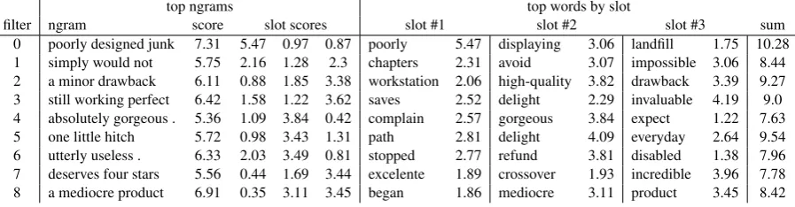
Table 1shows the top-scoring naturally occur-ring and possible ngrams for nine filters in the Elec model. In each of the top scoring natural ngrams, at least one slot receives a low activation. Table2
zooms in on one of the filters and shows its top-7 naturally occurring ngrams and top-top-7 most acti-vated words in each slot. Here, most top-scoring ngrams maximize slot #3 with words such as in-valuableandperfect, however some ngrams such as “worksas good” and “stillholdingstrong” max-imize slots #1 and #2 respectively, instead.
Additionally, most top-scoring words do not ap-pear to be utilized in high-scoring ngrams at all. This can be explained with the following: if a word such ascrtrarely or never appears in slot #1 alongside other high-scoring words in other slots, then crt can score highly with no consequence. Since an ngram containingcrtat slot #1 will rarely pass the max-pooling layer, its score at that slot is essentially random.
top ngrams top words by slot
filter ngram score slot scores slot #1 slot #2 slot #3 sum
0 poorly designed junk 7.31 5.47 0.97 0.87 poorly 5.47 displaying 3.06 landfill 1.75 10.28
1 simply would not 5.75 2.16 1.28 2.3 chapters 2.31 avoid 3.07 impossible 3.06 8.44
2 a minor drawback 6.11 0.88 1.85 3.38 workstation 2.06 high-quality 3.82 drawback 3.39 9.27
3 still working perfect 6.42 1.58 1.22 3.62 saves 2.52 delight 2.29 invaluable 4.19 9.0
4 absolutely gorgeous . 5.36 1.09 3.84 0.42 complain 2.57 gorgeous 3.84 expect 1.22 7.63
5 one little hitch 5.72 0.98 3.43 1.31 path 2.81 delight 4.09 everyday 2.64 9.54
6 utterly useless . 6.33 2.03 3.49 0.81 stopped 2.77 refund 3.81 disabled 1.38 7.96
7 deserves four stars 5.56 0.44 1.69 3.44 excelente 1.89 crossover 1.93 incredible 3.96 7.78
[image:6.595.75.524.64.181.2]8 a mediocre product 6.91 0.35 3.11 3.45 began 1.86 mediocre 3.11 product 3.45 8.42
Table 1: Top ngrams and words by filter from a sample of nine filters from the Elec model. The average difference between the top natural ngram activation and the top possible ngram activation for this model is 2.5, or a 30% average reduction.
top ngrams
rank ngram score slot scores
1 still workingperfect 6.42 1.58 1.22 3.62
2 works -perfect 5.78 1.91 0.25 3.62
3 isolation provesinvaluable 5.61 0.39 1.03 4.19
4 still nearperfect 5.6 1.58 0.4 3.62
5 still working great 5.45 1.58 1.22 2.65
6 worksas good 5.44 1.91 1.45 2.08
7 stillholdingstrong 5.37 1.58 1.81 1.98
top words by slot
slot #1 slot #2 slot #3
saves 2.52 delight 2.29 invaluable 4.19
crt 2.1 holding 1.81 perfect 3.62
beginner 2.09 welcome 1.8 cm 3.61
mics 2.08 dhcp 1.72 pleasant 3.38
genius 2.07 completely 1.64 simplicity 3.14
final 2.01 cradle 1.56 england 3.09
[image:6.595.75.527.240.341.2]works 1.91 well-made 1.51 daily 3.04
Table 2: Top-k words by slot scores and top-k ngrams by filter scores from the Elec model. In bold are words from the top-k ngrams which appear in the top-k slot words - i.e. words which maximize their slot.
(i) Each filter captures multiple semantic classes of ngrams, and each class has some domi-nating slots and some non-domidomi-nating slots (which we define as aslot activation pattern).
(ii) A slot may not be maximized because it’s not used to detect word existence, but rather lack of existence—ensuring that specific words do not occur.
We investigate both hypotheses in Sections5.3and
5.4respectively.
Adversarial potential We note in passing that this discrepancy in scores between naturally oc-curring and possible ngrams can be used to derive adversarial examples that cause a trained model to misclassify. By inserting a few seemingly ran-dom ngrams, we can cause filters to activate be-yond their expected range, potentially driving the model to misclassification. We reserve this area of exploration for future work.
5.3 Clustering (Hypothesis(i))
We explore hypothesis(i)by clustering threshold-passing (naturally occurring) ngrams in each fil-ter according to their activation vectors. We use Mean Shift Clustering (Fukunaga and Hostetler,
1975; Cheng, 1995), an algorithm that does not require specifying an a-priori number of clusters, and does not make assumptions about their shapes. Mean Shift considers the feature vectors as sam-pled from an underlying probability density func-tion6. Each cluster captures a different slot activa-tion pattern. We use the cluster’s centroid as the prototypical slot activation for that cluster.
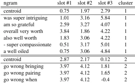
Table3shows a sample clustering output. The clustering algorithm identified two clusters: one primarily containing ngrams of the pattern DET INTENSITY-ADVERB POSITIVE-WORD, while the second contains ngrams that begin with phrases likego wrong.7
The centroids for these clusters capture the acti-vation patterns well: low-medium-high and high-high-low for clusters 1 and 2 respectively.
To summarize, by discarding noisy ngrams which do not pass the filter’s threshold and then clustering those that remain according to their slot activation patterns, we arrived at a clearer image
6Intuitively, we can think of the sampling noise as the ngram embeddings, and the probability distribution as de-fined by a function of the filter weights.
7In the Yelp dataset,
ngram slot #1 slot #2 slot #3 cluster
centroid 0.75 1.97 2.79 1
was super intriguing 1.01 3.16 5.84 1
am so grateful 2.59 3.27 4.07 1
overall very worth 3.84 1.86 4.22 1
also well worth 1.83 3.06 4.22 1
- super compassionate 0.51 3.17 5.01 1
a well oiled 0.75 3.06 4.84 1
centroid 2.87 2.17 0.12 2
go wrong bringing 3.97 4.12 1.81 2
go wrong pairing 3.97 4.12 1.65 2
[image:7.595.71.289.63.197.2]go wrong when 3.97 4.12 -0.4 2
Table 3: Example clustering results on the Yelp dataset. After applying thresholds, the ngrams for this filter were split into two clusters of sizes 83% and 17% re-spectively. The table shows top-scoring ngrams for this filter with their clustering results, sorted by their acti-vation strength.
of the semantic classes of ngrams that a given fil-ter specializes in capturing. In particular, we re-veal that filters are not necessarily homogeneous: a single filter may detect several different seman-tic patterns, each one of them relying on a different slot activation pattern.
5.4 Negative Ngrams (Hypothesis(ii))
Our second theory to explain the discrepancy be-tween the activations of naturally occurring and possible ngrams is that certain filter slots are not used to detect a class of highly activating words, but rather to rule out a class of highly negative words. We refer to these asnegative ngrams.
For example, Table 3 shows an ngram pattern for which slot #1 contains determiners and other “filler” tokens such as hyphens, periods and com-mas with relatively weak slot activations. Hypoth-esis(ii)suggests that this slot may receive a strong negativescore for words such asnotandn’t, caus-ing such negated patterns to drop below the thresh-old. Indeed, ngrams containingnotorn’tin slot #1 do not pass the threshold for this filter.
We are interested in a more systematic method of identifying these cases. Identifying negative slot activations would be very useful for under-standing the semantics captured by a filter and the reasoning behind the dismissal of an ngram, as we discuss in Sections6.1and6.2respectively.
We achieve this by searching the below-threshold ngram space for ngrams which are “flipped versions” of above-threshold ngrams. Concretely: Given ngram u which was scored highly by filter f, we search for low-scoring
ngrams u0 such that the hamming distance be-tweenuandu0 is low. By doing this for the top-k scoring ngrams per cluster, we arrive at a com-prehensive set of negative ngrams. In Table4we show a sample output of this algorithm.
Furthermore, we can divide negative ngrams into two cases: 1) Lowering the ngram score be-low the threshold by replacing high-scoring words with low-scoring words. 2) Lowering the ngram score below the threshold by replacing words with a low positive score with words with a highly-neg-ative score. Case 2 is more interesting because it embodies cases where hypothesis (ii) is rele-vant. Additionally, it highlights ngrams where a strongly positive word in one slot was negated with another strongly negative word in another slot. Table4shows examples in bold.
In order to identify “Case 2” negative ngrams, we heuristically test whether the “changed” words’ scores directly influence the status of the activation relative to the threshold: given an al-ready identified negative ngram, if the ngram score—sans the bottom-k negative slot activations (considering a hamming distance ofk and given that there areknegative slot activations)—passes the threshold, yet it does not pass the threshold by including the negative slot activations, then the ngram is considered a “Case 2” negative ngram.
6 Interpretability
In this section we show two practical implica-tions of the findings above: improvements in both model-level and prediction-level interpretability of 1D CNNs for text classification.
6.1 Model Interpretability
ngram slot #1 slot #2 slot #3 sum
’m really pleased 2.59 1.86 5.05 9.5
’m really not -2.49 1.96
’m really upset -1.14 3.31
’m not pleased -3.4 4.24
is extremely useful 2.3 3.24 3.96 9.5
is extremely limited -2.8 2.74
is extremely noisy -2.77 2.8
is not useful -3.4 2.86
is only useful -2.82 3.44
is surprisingly good 2.3 4.32 2.8 9.42
is not good -3.4 1.7
is only good -2.82 2.28
is no good -1.88 3.22
is probably good -1.66 3.44
am very satisfied 2.01 2.17 5.09 9.26
am very dissatisfied -1.9 2.27
am very disappointed -1.87 2.3
am not satisfied -3.4 3.69
[image:8.595.310.526.83.203.2]not very satisfied -2.6 4.66
Table 4: Top-scoring ngrams from one filter from a model trained on the Elec dataset, and their accompa-nying lowest-scoring negative ngrams. We selected a hamming distance of 1 word. Bold ngrams are Case 2 negative ngrams.
slot-activation vector, and its list of bottom-k neg-ative ngrams with their activations and slot acti-vations. In particular, by clustering the activated ngrams according to their slot activation patterns and showing the top-k in each clusters, we get a much more refined coverage of the linguistic pat-terns that are captured by the filter.
6.2 Prediction Interpretability
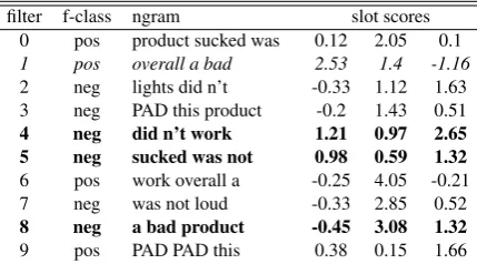
Previous prediction-based interpretation attempts traced back the ngrams from the max-pooling layer. Here we improve these previous attempts by considering only ngrams that pass the threshold for their filter. This results in a more concise and relevant explanation (Figure 1). Figure 3 shows two examples. Note that in example #1, many negative-class filters were “forced” to choose an ngram in max-pooling despite there not being strongly negative phrases—but those ngrams do not pass the threshold and are thus cleaned from the explanation.
Additionally we can use the individual slot ac-tivations to tease-apart the contribution of each word in the ngram. Finally, we can also mark cases of negative-ngrams (Section5.4), where an ngram has high slot activations for some words, but these are negated by a highly-negative slot and
myUNK fits perfectly . very wellmade . nice looking and offers good protection
filter f-class ngram slot scores
0 pos PAD PAD my 0.7 1.65 0.16
1 pos . very well 0.98 2.17 2.63
2 neg PAD my UNK 1.31 -0.07 0.21
3 neg UNK fits perfectly 0.28 0.61 0.03
4 neg looking and offers 0.6 0.12 0.5
5 neg good protection PAD 0.52 1.6 -0.01
6 pos UNK fits perfectly -0.06 2.36 1.82
7 neg fits perfectly . 1.34 -0.71 1.47
8 neg . very well -0.01 1.97 -0.55
9 pos perfectly . very 4.13 0.45 -0.01
this productsucked was notloud at all lightsdid n’t work overalla badproductthat ’s UNK taking up space
filter f-class ngram slot scores
0 pos product sucked was 0.12 2.05 0.1
1 pos overall a bad 2.53 1.4 -1.16
2 neg lights did n’t -0.33 1.12 1.63
3 neg PAD this product -0.2 1.43 0.51
4 neg did n’t work 1.21 0.97 2.65 5 neg sucked was not 0.98 0.59 1.32
6 pos work overall a -0.25 4.05 -0.21
7 neg was not loud -0.33 2.85 0.52
8 neg a bad product -0.45 3.08 1.32
9 pos PAD PAD this 0.38 0.15 1.66
Figure 3: Examples predicted positive and negative respectively by a model trained on the Elec dataset, along with their explanations. Ngrams which passed the threshold are in bold, and case 2 negative ngrams are in italics. For clarity’s sake we trained a small model which uses ten filters.
as a consequence are not selected by max-pooling, or are selected but do not pass the filter’s thresh-old.
7 Conclusion
[image:8.595.309.524.233.352.2]the word-level, but instead form slot activation patterns that give different types of ngrams similar activation strengths. This provides empirical evi-dence that filters are not homogeneous. By clus-tering high-scoring ngrams according to their slot-activation patterns we can identify the groups of linguistic patterns captured by a filter. We also show that filters sometimes opt to assign nega-tive values to certain word activations in order to cause the ngrams which contain them to receive a low score despite having otherwise highly activat-ing words. Finally, we use these findactivat-ings to sug-gest improvements to model-based and prediction-based interpretability of CNNs for text.
References
David Alvarez-Melis and Tommi S. Jaakkola. 2017. A causal framework for explaining the predic-tions of black-box sequence-to-sequence models. In Proceedings of the 2017 Conference on Em-pirical Methods in Natural Language Processing, EMNLP 2017, Copenhagen, Denmark, September 9-11, 2017, pages 412–421. Association for Com-putational Linguistics.
Shaojie Bai, J. Zico Kolter, and Vladlen Koltun. 2018. An empirical evaluation of generic convolu-tional and recurrent networks for sequence model-ing. CoRR, abs/1803.01271.
Yizong Cheng. 1995. Mean shift, mode seeking, and clustering. IEEE Trans. Pattern Anal. Mach. Intell., 17(8):790–799.
Ronan Collobert, Jason Weston, L´eon Bottou, Michael Karlen, Koray Kavukcuoglu, and Pavel P. Kuksa. 2011. Natural language processing (almost) from scratch. Journal of Machine Learning Research, 12:2493–2537.
Keinosuke Fukunaga and Larry D. Hostetler. 1975. The estimation of the gradient of a density func-tion, with applications in pattern recognition. IEEE Trans. Information Theory, 21(1):32–40.
Yoav Goldberg. 2016. A primer on neural network models for natural language processing. J. Artif. In-tell. Res., 57:345–420.
Pei Guo, Connor Anderson, Kolten Pearson, and Ryan Farrell. 2018. Neural network interpreta-tion via fine grained textual summarizainterpreta-tion. CoRR, abs/1805.08969.
Mohit Iyyer, Varun Manjunatha, Jordan L. Boyd-Graber, and Hal Daum´e III. 2015. Deep unordered composition rivals syntactic methods for text clas-sification. InProceedings of the 53rd Annual Meet-ing of the Association for Computational LMeet-inguistics
and the 7th International Joint Conference on Nat-ural Language Processing of the Asian Federation of Natural Language Processing, ACL 2015, July 26-31, 2015, Beijing, China, Volume 1: Long Pa-pers, pages 1681–1691. The Association for Com-puter Linguistics.
Rie Johnson and Tong Zhang. 2015. Effective use of word order for text categorization with convolu-tional neural networks. InNAACL HLT 2015, The 2015 Conference of the North American Chapter of the Association for Computational Linguistics: Human Language Technologies, Denver, Colorado, USA, May 31 - June 5, 2015, pages 103–112. The Association for Computational Linguistics.
Nal Kalchbrenner, Edward Grefenstette, and Phil Blun-som. 2014. A convolutional neural network for modelling sentences. In Proceedings of the 52nd Annual Meeting of the Association for Computa-tional Linguistics, ACL 2014, June 22-27, 2014, Baltimore, MD, USA, Volume 1: Long Papers, pages 655–665. The Association for Computer Linguis-tics.
Yoon Kim. 2014. Convolutional neural networks for sentence classification. InProceedings of the 2014 Conference on Empirical Methods in Natural Lan-guage Processing, EMNLP 2014, October 25-29, 2014, Doha, Qatar, A meeting of SIGDAT, a Special Interest Group of the ACL, pages 1746–1751. ACL.
Yann LeCun, Y Bengio, and Geoffrey Hinton. 2015. Deep learning. 521:436–44.
Yann LeCun, Leon Bottou, Y Bengio, and Patrick Haffner. 1998. Gradient-based learning applied to document recognition. 86:2278 – 2324.
Tao Lei, Regina Barzilay, and Tommi S. Jaakkola. 2016. Rationalizing neural predictions. In Pro-ceedings of the 2016 Conference on Empirical Meth-ods in Natural Language Processing, EMNLP 2016, Austin, Texas, USA, November 1-4, 2016, pages 107–117. The Association for Computational Lin-guistics.
Julian J. McAuley and Jure Leskovec. 2013. Hidden factors and hidden topics: understanding rating di-mensions with review text. InSeventh ACM Confer-ence on Recommender Systems, RecSys ’13, Hong Kong, China, October 12-16, 2013, pages 165–172. ACM.
Julian J. McAuley, Christopher Targett, Qinfeng Shi, and Anton van den Hengel. 2015. Image-based rec-ommendations on styles and substitutes. In Pro-ceedings of the 38th International ACM SIGIR Con-ference on Research and Development in Informa-tion Retrieval, Santiago, Chile, August 9-13, 2015, pages 43–52. ACM.
Jeffrey Pennington, Richard Socher, and Christo-pher D. Manning. 2014. Glove: Global vectors for word representation. InEmpirical Methods in Nat-ural Language Processing (EMNLP), pages 1532– 1543.
Marco T´ulio Ribeiro, Sameer Singh, and Carlos Guestrin. 2016. ”why should I trust you?”: Explain-ing the predictions of any classifier. In Proceed-ings of the 22nd ACM SIGKDD International Con-ference on Knowledge Discovery and Data Mining, San Francisco, CA, USA, August 13-17, 2016, pages 1135–1144. ACM.
Avraham Ruderman, Neil C. Rabinowitz, Ari S. Mor-cos, and Daniel Zoran. 2018. Learned deformation stability in convolutional neural networks. CoRR, abs/1804.04438.
Peng Wang, Jiaming Xu, Bo Xu, Cheng-Lin Liu, Heng Zhang, Fangyuan Wang, and Hongwei Hao. 2015. Semantic clustering and convolutional neural net-work for short text categorization. In Proceed-ings of the 53rd Annual Meeting of the Association for Computational Linguistics and the 7th Interna-tional Joint Conference on Natural Language Pro-cessing of the Asian Federation of Natural Language Processing, ACL 2015, July 26-31, 2015, Beijing, China, Volume 2: Short Papers, pages 352–357. The Association for Computer Linguistics.
Matthew D. Zeiler and Rob Fergus. 2014. Visualizing and understanding convolutional networks. In Com-puter Vision - ECCV 2014 - 13th European Con-ference, Zurich, Switzerland, September 6-12, 2014, Proceedings, Part I, volume 8689 ofLecture Notes in Computer Science, pages 818–833. Springer.