Using LTAG Based Features in Parse Reranking
∗Libin Shen
Dept. of Computer & Info. Sci. University of Pennsylvania
Anoop Sarkar
School of Computing Science Simon Fraser University
Aravind K. Joshi
Dept. of Computer & Info. Sci. University of Pennsylvania
Abstract
We propose the use of Lexicalized Tree Adjoining Grammar (LTAG) as a source of features that are useful for reranking the output of a statistical parser. In this paper, we extend the notion of a tree ker-nel over arbitrary sub-trees of the parse to the derivation trees and derived trees pro-vided by the LTAG formalism, and in ad-dition, we extend the original definition of the tree kernel, making it more lexi-calized and more compact. We use LTAG based features for the parse reranking task and obtain labeled recall and precision of
89.7%/90.0%on WSJ section 23 of Penn
Treebank for sentences of length ≤ 100 words. Our results show that the use of LTAG based tree kernel gives rise to a 17% relative difference in f-score im-provement over the use of a linear kernel without LTAG based features.
1 Introduction
Recent work in statistical parsing has explored al-ternatives to the use of (smoothed) maximum likeli-hood estimation for parameters of the model. These alternatives are distribution-free (Collins, 2001), providing a discriminative method for resolving parse ambiguity. Discriminative methods provide a rankingbetween multiple choices for the most plau-sible parse tree for a sentence, without assuming that a particular distribution or stochastic process gener-ated the alternative parses.
∗We would like to thank Michael Collins for providing the
originaln-best parsed data on which we ran our experiments
and the anonymous reviewers for their comments. The sec-ond author is partially supported by NSERC, Canada (RGPIN: 264905).
Discriminative methods permit the use of feature functions that can be used to condition on arbitrary aspects of the input. This flexibility makes it possi-ble to incorporate features of various of kinds. Fea-tures can be defined on characters, words, part of speech (POS) tags and context-free grammar (CFG) rules, depending on the application to which the model is applied.
Features defined on n-grams from the input are the most commonly used for NLP applications. Such n-grams can either be defined explicitly us-ing some lus-inguistic insight into the problem, or the model can be used to search the entire space ofn -gram features using a kernel representation. One example is the use of a polynomial kernel over se-quences. However, to use all possible n-gram fea-tures typically introduces too many noisy feafea-tures, which can result in lower accuracy. One way to solve this problem is to use a kernel function that is tailored for particular NLP applications, such as the tree kernel (Collins and Duffy, 2001) for statistical parsing.
scope of previous tree kernel definitions using arbi-trary sub-trees. In this paper, we use the LTAG based features in the parse reranking problem (Collins, 2000; Collins and Duffy, 2002). We use the Sup-port Vector Machine (SVM) (Vapnik, 1999) based algorithm proposed in (Shen and Joshi, 2003) as the reranker in this paper. We apply the tree kernel to derivation trees of LTAG, and extract features from derivation trees. Both the tree kernel and the linear kernel on the richer feature set are used. Our exper-iments show that the use of tree kernel on derivation trees makes the notion of a tree kernel more power-ful and more applicable.
2 Lexicalized Tree Adjoining Grammar In this section, we give a brief introduction to the Lexicalized Tree Adjoining Grammar (more details can be found in (Joshi and Schabes, 1997)). In LTAG, each word is associated with a set of elemen-tary trees. Each elementary tree represents a possi-ble tree structure for the word. There are two kinds of elementary trees,initial treesandauxiliary trees. Elementary trees can be combined through two op-erations,substitutionandadjunction. Substitution is used to attach an initial tree, and adjunction is used to attach an auxiliary tree. In addition to adjunction, we also usesister adjunctionas defined in the LTAG statistical parser described in (Chiang, 2000).1 The
tree resulting from the combination of elementary trees is is called aderived tree. The tree that records the history of how a derived tree is built from the elementary trees is called aderivation tree.2
We illustrate the LTAG formalism using an exam-ple.
Example 1: Pierre Vinken will join the board as a non-executive director.
The derived tree for Example 1 is shown in Fig. 1 (we omit the POS tags associated with each word to save space), and Fig. 2 shows the elementary trees for each word in the sentence. Fig. 3 is the deriva-tion tree (the history of tree combinaderiva-tions). One of
1Adjunction is used in the case where both the root node and
the foot node appear in the Treebank tree. Sister adjunction is used in generating modifier sub-trees as sisters to the head, e.g in basal NPs.
2Each nodeηhniin the derivation tree is an elementary tree
nameηalong with the locationnin the parent elementary tree
whereηis inserted. The locationnis the Gorn tree address (see
Fig. 4).
S
NP
Pierre Vinken
VP
will VP
VP
join NP
the board
PP
as NP
[image:2.612.318.534.70.178.2]a non-executive director
Figure 1: Derived tree (parse tree) for Example 1.
NP
Pierre NP
Vinken
VP
will VP∗
S
NP↓ VP
join NP↓
NP
the
NP
board
VP
VP∗ PP
as NP↓
NP
a
NP
non-executive NP
director
β1: α2: β2: α1:
β3: α3: β4: β6: β5: α4:
Figure 2: Elementary trees for Example 1.
the properties of LTAG is that it factors recursion in clause structure from the statement of linguistic con-straints, thus making these constraints strictly local. For example, in the derivation tree of Examples 1, α1(join) and α2(V inken) are directly connected
whether there is an auxiliary tree β2(will) or not.
We will show how this property affects our redefined tree kernel later in this paper. In our experiments in this paper, we only use LTAG grammars where each elementary tree is lexicalized by exactly one word (terminal symbol) on the frontier.
3 Parse Reranking
In recent years, reranking techniques have been suc-cessfully used in statistical parsers to rerank the out-put of history-based models (Black et al., 1993). In this paper, we will use the LTAG based features to improve the performance of reranking. Our motiva-tions for using LTAG based features for reranking are the following:
[image:2.612.313.543.219.334.2]α1(join)hi
α2(Vinken)h00i
β1(Pierre)h0i
β2(will)h01i α3(board)h011i
β3(the)h0i
β4(as)h01i
α4(director)h011i
β5(non-executive)h0i
[image:3.612.71.453.74.166.2]β6(a)h0i
Figure 3: Derivation tree: shows how the elementary trees shown in Fig. 2 can be combined to provide an analysis for the sentence in Example 1.
which allow us tocombinefeatures that are de-fined on arbitrary sub-trees in the parse tree and features defined on a derivation tree.
• Several hand-crafted and arbitrary features have been exploited in the statistical parsing task, especially when parsing the WSJ Penn Treebank dataset where performance has been finely tuned over the years. Showing a positive contribution in this task will be a convincing test for the use of LTAG based features.
• The parse reranking dataset is well established. We use the dataset defined in (Collins, 2000).
In (Collins, 2000), two reranking algorithms were proposed. One was based on Markov Random Fields, and the other was based on the Boosting al-gorithm. In both these models, the loss functions were computed directly on the feature space. Fur-thermore, a rich feature set was introduced that was specifically selected by hand to target the limitations of generative models in statistical parsing.
In (Collins and Duffy, 2002), the Voted Percep-tron algorithm was used for parse reranking. The
S0
NP00
↓ VP
01
join010 NP011
↓
Figure 4: Example of how each node in an elemen-tary tree has a unique node address using the Gorn notation. 0is the root with daughters00,01, and so
on recursively, e.g. first daughter01is010.
VP
will VP
... PP ... NP
a
Figure 5: A sub-tree which is linguistically mean-ingless.
tree kernel was used to compute the number of com-mon sub-trees of two parse trees. The features used by this tree kernel contains all the hand selected fea-tures of (Collins, 2000). It is worth mentioning that thef-scores reported in (Collins and Duffy, 2002) are about1%less than the results in (Collins, 2000).
In (Shen and Joshi, 2003), a SVM based rerank-ing algorithm was proposed. In that paper, the no-tion of preference kernels was introduced to solve the reranking problem. Two distinct kernels, the tree kernel and the linear kernel were used with prefer-ence kernels.
4 Using LTAG Based Features 4.1 Motivation
While the tree kernel is an easy way to compute sim-ilarity between two parse trees, it takes too many lin-guistically meaningless sub-trees into consideration. Let us consider the example sentence in Example 1. The parse tree, or derived tree, for this sentence is shown in Fig. 1. Fig. 5 shows one of the lin-guistically meaningless sub-trees. The number of meaningless sub-trees is a misleading measure for discriminating good parse trees from bad. Further-more, the number of meaningless sub-trees is far greater than the number of useful sub-trees. This limits both efficiency and accuracy on the test data. The use of unwanted sub-trees greatly increases the hypothesis spaceof a learning machine, and thus de-creases the expected accuracy on test data. In this work, we consider the hypothesis that linguistically meaningful sub-trees reveal correlations of interest and therefore are useful in stochastic models.
provide a more accurate measure of similarity be-tween two parses. This is one of the motivations for applying tree kernels to derivation trees. Note that the use of features on derivation trees is differ-ent from the use of features on dependency graphs, derivation trees include many complex patterns of tree names and attachment sites and can represent word to word dependencies that are not possible in traditional dependency graphs.
For example, the derivation tree for Example 1 with and without optional modifiers such asβ4(as)
are minimally different. In contrast, in derived (parse) trees, there is an extra VP node which changes quite drastically the set of sub-trees with and without the PP modifier. In addition, using only sub-trees from the derived tree, we cannot repre-sent a common sub-tree that contains only the words Vinkenandjoinsince this would lead to a discontin-uoussub-tree. However, LTAG based features can represent such cases trivially.
The comparison between (Collins, 2000) and (Collins and Duffy, 2002) in§3 shows that it is hard to add new features to improve performance. Our hypothesis is that the LTAG based features provide a novel set of abstract features that complement the hand selected features from (Collins, 2000) and the LTAG based features will help improve performance in parse reranking.
4.2 Extracting Derivation Trees
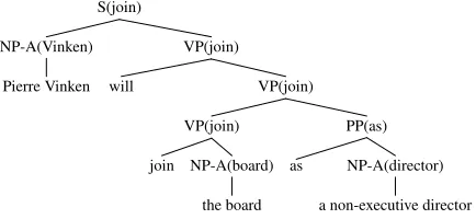
Before we can use LTAG based features we need to obtain an LTAG derivation tree for each parse tree under consideration by the reranker. Our solu-tion is to extract elementary trees and the derivasolu-tion tree simultaneously from the parse trees produced by an n-best statistical parser. Our training and test data consists ofn-best output from the Collins parser (see (Collins, 2000) for details on the dataset). Since the Collins parser uses a lexicalized context-free grammar as a basis for its statistical model, we obtain parse trees that are of the type shown in Fig. 6. From this tree we extract elementary trees and derivation trees by recursively traversing the spine of the parse tree. The spine is the path from a non-terminal lexicalized by a word to the non-terminal sym-bol on the frontier equal to that word. Every sub-tree rooted at a non-terminal lexicalized by a different word is excised from the parse tree and recorded into
S(join)
NP-A(Vinken)
Pierre Vinken
VP(join)
will VP(join)
VP(join)
join NP-A(board)
the board
PP(as)
as NP-A(director)
[image:4.612.319.536.72.172.2]a non-executive director
Figure 6: Sample output parse from the Collins parser. Each non-terminal is lexicalized by the pars-ing model. -A marks arguments recovered by the parser.
the derivation tree as asubstitution. Repeated non-terminals on the spine (e.g. VP(join). . .VP(join) in Fig. 6) are excised along with the sub-trees hang-ing off of it and recorded into the derivation tree as an adjunction. The only other case is those sub-trees rooted at non-terminals that are attached to the spine. These sub-trees are excised and recorded into the derivation tree as cases ofsister adjunction. Each sub-tree excised is recursively analyzed with this method, split up into elementary trees and then recorded into the derivation tree. The output of our algorithm for the input parse tree in Fig. 6 is shown in Fig. 2 and Fig. 3. Our algorithm is similar to the derivation tree extraction explained in (Chiang, 2000), except we extract our LTAG fromn-best sets of parse trees, while in (Chiang, 2000) the LTAG is extracted from the Penn Treebank.3 For other
tech-niques for LTAG grammar extraction see (Xia, 2001; Chen and Vijay-Shanker, 2000).
4.3 Using Derivation Trees
In this paper, we have described two models to em-ploy derivation trees. Model 1 uses tree kernels on derivation trees. In order to make the tree kernel more lexicalized, we extend the original definition of the tree kernel, which we will describe below. Model 2 abstracts features from derivation trees and uses them with a linear kernel.
In Model 1, we combine the SVM results of the tree kernel on derivation trees with the SVM results given by a linear kernel based on features on the de-rived trees.
3Also note that the path from the root node to the foot node
In Model 2, the vector space of the linear kernel consists of both LTAG based features defined on the derived trees and features defined on the derivation tree. The following LTAG features have been used in Model 2.
• Elementary tree. Each node in the derivation tree is used as a feature.
• Bigram of parent and its child. Each pair of parent elementary tree and child elementary tree, as well as the type of operation (substi-tution, adjunction or sister adjunction) and the Gorn address on parent (see Fig. 4) is used as a feature.
• Lexicalized elementary tree. Each elemen-tary tree associated with its lexical item is used as a feature.
• Lexicalized bigram. InBigram of parent and its child, each elementary tree is lexicalized (we use closed class words, e.g. adj, adv, prep, etc. but not noun or verb).
4.4 Lexicalized Tree Kernel
In (Collins and Duffy, 2001), the notion of a tree ker-nel is introduced to compute the number of common sub-trees of two parse trees. For two parse trees,p1
andp2, the tree kernelTree(p1, p2) is defined as:
Tree(p1, p2) =
X
n1in p1
n2in p2
T(n1, n2) (1)
The recursive functionT is defined as follows: Ifn1
andn2have the same bracketing tag (e.g. S, NP, VP,
. . .) and the same number of children,
T(n1, n2) =λ Y
i
(1 +T(n1i, n2i)), (2)
where, nki is the ith child of the node nk, λ is a
weight coefficient used to control the importance of large sub-trees and0< λ≤1.
Ifn1andn2have the same bracketing tag but
dif-ferent number of children, T(n1, n2) = λ. If they
don’t have the same bracketing tag,T(n1, n2) = 0.
In (Collins and Duffy, 2002), lexical items are all located at the leaf nodes of parse trees. Therefore
VP(join)
VP(join)
V(join) NP(board)
PP(as)
P(as) NP(director) tree with root noden:
VP
VP
V NP PP
P NP ptn(n):
[image:5.612.341.512.71.204.2]lex(n): (join, join, as)
Figure 7: A lexicalized sub-tree rooted at n and its decomposition into a pattern, ptn(n) and corre-sponding vector of lexical information, lex(n).
sub-trees that do not contain any leaf node are not lexicalized. Furthermore, due to the introduction of parameter λ, lexical information is almost ignored for sub-trees whose root node is not close to the leaf nodes, i.e. sub-trees rooted atSnode.
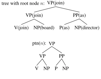
In order to make the tree kernel more lexicalized, we associate each node with a lexical item. For ex-ample, Fig. 7 shows a lexicalized sub-tree and its decomposition into features. As shown in Fig. 7 the lexical informationlex(t)extracted from the lexical-ized tree consists of words from the root and its im-mediate children. This is because we wish to ig-nore irrelevant lexicalizations such asNP(board)in Fig. 7.
A lexicalized sub-tree rooted on node n is split into two parts. One is the pattern tree ofn,ptn(n).
The other is the vector of lexical information ofn, lex(n), which contains the lexical items of the root node and the children of the root.
For two tree nodesn1andn2, the recursive
func-tionLT(n1, n2)used to compute the lexicalized tree
kernel is defined as follows.
LT(n1, n2) = (1 +Cnt(lex(n1), lex(n2)))
× T0(ptn(n
1), ptn(n2)), (3)
whereT0 is the same as the original recursive
func-tion T defined in (2), except that T is defined on parse tree nodes, while T0 is defined on patterns of
parse tree nodes. Cnt(x, y) counts the number of
2 elements of the two vectors are the same.
It can be shown that the lexicalized tree kernel counts the number of common sub-trees that meet the following constraints.
• None or one node in the sub-tree is lexicalized
• The lexicalized node is the root node or a child of the root, if applicable.
Therefore our new tree kernel is more lexicalized. On the other hand, it immediately follows that the lexicalized tree kernel is well-defined. It means that we can embed the lexicalized tree kernel into a high dimensional space. The proof is similar to the proof for the tree kernel in (Collins and Duffy, 2001).
Another important advantage of the lexicalized tree kernel is that it is more compressible. It is noted in (Collins and Duffy, 2001) that training trees can be combined by sharing sub-trees to speed up the test. As far as the lexicalized tree kernel is con-cerned, the pattern trees are more compressible be-cause there is no lexical item at the leaf nodes of pattern trees. Lexical information can be attached to the nodes of the result pattern forest. In our ex-periment, we select five parses from each sentence in Collins’ training data and represent these parses with shared structure. The number of the nodes in the pattern forest is only 1/7 of the total number of the nodes the selected parse trees.
4.5 Tree Kernel for Derivation Trees
In order to apply the (lexicalized) tree kernel to derivation trees, we need to make some modifica-tions to the original recursive definition of the tree kernel.
For derivation trees, the recursive function is trig-gered if the two root nodes have the same non-lexicalized elementary tree (sometimes called su-pertag). Note that these two nodes will have the same number of children which are initial trees (aux-iliary trees are not counted). In comparison, the re-cursive function in (2),T(n1, n2)is computed if and
only ifn1 andn2 have the same bracketing tagand
they have the same number of children.
For each node, its children are attached with one of the two distinct operations, substitution or adjunc-tion. For substituted children, the computation of the tree kernel is almost the same as that for CFG parse
tree. However, there is a problem with the adjoined children. Let us first have a look at a sentence in Penn Treebank.
Example 2: COMMERCIAL PAPER placed di-rectly by General Motors Acceptance Corp.: 8.55%
30 to 44 days; 8.25%45 to 59 days; 8.45%60 to 89
days; 8%90 to 119 days; 7.90%120 to 149 days;
7.80%150 to 179 days; 7.55%180 to 270 days. In this example, seven sub-trees of the same type are sister adjoined to the same place of an initial tree. So the number of common sub-trees increases dra-matically if the tree kernel is applied on two similar parses of this sentence. Experimental evidence indi-cates that this is harmful to accuracy. Therefore, for derivation trees, we are only interested in sub-trees that contain at most 2 adjunction branches for each node. The number of constrained common sub-trees for the derivation tree kernel can be computed by the recursive functionDT over derivation tree nodes n1, n2:
DT(n1, n2) = (1 +A1(n1, n2) +A2(n1, n2))
× T”(sub(n1), sub(n2)) (4)
wheresub(nk) is the sub-tree ofnk in which
chil-dren adjoined to the root of nk are pruned. T” is
similar to the original recursive function T defined in (2), but it is defined on derivation tree nodes re-cursively. A1 andA2are used to count the number
of common sub-trees whose root nodes only contain one or two adjunction children respectively.
A1(n1, n2) = X
i,j
DT(a1i, a2j),
where,a1iis theith adjunct ofn1, anda2j is thejth
adjunct ofn2. Similarly, we have:
A2(n1, n2) = X
i<k,j<l
DT(a1i, a2j)·DT(a1k, a2l)
The tree kernel for derivation trees is a well-defined kernel function because we can easily define an em-bedding space according to the definition of the new tree kernel. By substitutingDTforT0in (3), we
ob-tain the lexicalized tree kernel for LTAG derivation trees (usingLT in (1)).
5 Experiments
experiments. We use preference kernels and pair-wise parse trees in our reranking models.
We use the same data set as described in (Collins, 2000). Section 2-21 of the Penn WSJ Treebank are used as training data, and section 23 is used for fi-nal test. The training data contains around 40,000 sentences, each of which has 27 distinct parses on average. Of the 40,000 training sentences, the first 36,000 are used to train SVMs. The remaining 4,000 sentences are used as development data.
Due to the computational complexity of SVM, we have to divide training data into slices to speed up training. Each slice contain two pairs of parses from every sentence. Specifically, slice i contains pos-itive samples ((˜pk, pki),+1) and negative samples
((pki,p˜k),−1), wherep˜k is the best parse for
sen-tence k, pki is the parse with the ith highest
log-likelihood in all the parses for sentence k and it is not the best parse (Shen and Joshi, 2003). There are about 60000 samples in each slice in average.
For the tree kernel SVMs of Model 1, we take 3 slices as a chunk, and train an SVM for each chunk. Due to the limitation of computing resource, we have only trained on 3 chunks. The results of tree kernel SVMs are combined with simple com-bination. Then the outcome is combined with the result of the linear kernel SVMs trained on features extracted from the derived trees which are reported in (Shen and Joshi, 2003). For each parse, the num-ber of the brackets in it and the log-likelihood given by Collins’ parserModel 2are also used in the com-putation of the score of a parse. For each parsep, its scoreSco(p)is defined as follows:
Sco(p) =MT(p) +γ·ML(p) +β·l(p) +α·b(p),
whereMT(p)is the output of the tree kernel SVMs,
ML(p)is the output of linear kernel SVMs,l(p) is
the log-likelihood of parsep, and b(p) is the
num-ber of brackets in parsep. We noticed that the SVM systems prefers to give higher scores to the parses with less brackets. As a result, the system has a high precision but a low recall. Therefore, we take the number of brackets, b(p), as a feature to make the
recall and precision balanced. The three weight pa-rameters are tuned on the development data.
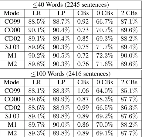
The results are shown in Table 1. With Model 1, we achieve LR/LP of89.7%/90.0%on sentences
≤40 Words (2245 sentences)
Model LR LP CBs 0 CBs 2 CBs
CO99 88.5% 88.7% 0.92 66.7% 87.1%
CO00 90.1% 90.4% 0.73 70.7% 89.6%
CD02 89.1% 89.4% 0.85 69.3% 88.2%
SJ 03 89.9% 90.3% 0.75 71.7% 89.4%
M1 90.2% 90.5% 0.72 72.3% 90.0%
M2 89.8% 90.3% 0.76 71.6% 89.6%
≤100 Words (2416 sentences)
Model LR LP CBs 0 CBs 2 CBs
CO99 88.1% 88.3% 1.06 64.0% 85.1%
CO00 89.6% 89.9% 0.87 68.3% 87.7%
CD02 88.6% 88.9% 0.99 66.5% 86.3%
SJ 03 89.4% 89.8% 0.89 69.2% 87.6%
M1 89.7% 90.0% 0.86 70.0% 88.2%
[image:7.612.313.547.72.297.2]M2 89.3% 89.8% 0.89 69.1% 87.7%
Table 1: Results on section 23 of the WSJ Tree-bank. LR/LP = labeled recall/precision. CBs = av-erage number of crossing brackets per sentence. 0 CBs, 2 CBs are the percentage of sentences with 0 or ≤ 2 crossing brackets respectively. CO99 = (Collins, 1999) Model 2. CO00 = (Collins, 2000). CD02 = (Collins and Duffy, 2002). SJ03 = linear kernel of (Shen and Joshi, 2003). M1=Model 1. M2=Model 2.
with ≤ 100 words. Our results show a 17% rel-ative difference in f-score improvement over the use of a linear kernel without LTAG based features (Shen and Joshi, 2003). In addition, we also get non-trivial improvement on the number of crossing brackets. These results verify the benefit of using LTAG based features and confirm the hypothesis that LTAG based features provide a novel set of abstract features that complement the hand selected features from (Collins, 2000). Our results on Model 1 show a1%error reduction on the previous best reranking
result using the dataset reported in (Collins, 2000). Also, Model 1 provides a 10% reduction in error over (Collins and Duffy, 2002) where the features from tree kernel were over arbitrary sub-trees.
0.874 0.875 0.876 0.877 0.878 0.879 0.88 0.881
0 5 10 15 20
ID of slices without LTAG
[image:8.612.79.300.68.209.2]with LTAG
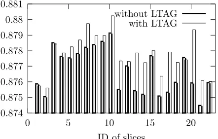
Figure 8: Comparison of performance of individual SVMs in Model 2: with and without LTAG based features. X-axis stands for the ID of the slices on which the SVMs are trained.Y-axis stands for thef -score.
improvement on most of the single SVMs, as shown in Fig. 8.
We think there are several reasons to account for why our Model 2 doesn’t work as well for the full task when compared with Model 1. Firstly, the train-ing slice is not large enough. Local optimization on each slice does not result in global optimization (as seen in Fig. 8). Secondly, the LTAG based features that we have used in the linear kernel in Model 2 are not as useful as the tree kernel in Model 1.4 The last
reason is that we do not set the importance of LTAG based features. One shortcoming of kernel methods is that the coefficient of each feature must be set be-fore the training (Herbrich, 2002). In our case, we do not tune the coefficients for the LTAG based fea-tures in Model 2.
6 Conclusions and Future Work
In this paper, we have proposed methods for using LTAG based features in the parse reranking task. The experimental results show that the use of LTAG based features gives rise to improvement over al-ready finely tuned results. We used LTAG based fea-tures for the parse reranking task and obtain labeled recall and precision of 89.7%/90.0% on WSJ
sec-tion 23 of Penn Treebank for sentences of length≤ 100 words. Our results show that the use of LTAG
4In Model 1, we implicitly take every sub-tree of the
deriva-tion trees as a feature, but in Model 2, we only consider a small set of sub-trees in a linear kernel.
based tree kernel gives rise to a17%relative
differ-ence inf-score improvement over the use of a linear kernel without LTAG based features. In future work, we will use some light-weight machine learning al-gorithms for which training is faster, such as vari-ants of the Perceptron algorithm. This will allow us to use larger training data chunks and take advan-tage of global optimization in the search for relevant features.
References
E. Black, F. Jelinek, J. Lafferty, Magerman D. M., R. Mercer, and S. Roukos. 1993. Towards history-based grammars: Using richer models for probabilistic parsing. InProc. of the ACL 1993.
R. Bod. 2003. An Efficient Implementation of a New DOP Model. InProc. of EACL 2003, Budapest.
J. Chen and K. Vijay-Shanker. 2000. Automated Extraction of TAGs from the Penn Treebank. InProc. of the 6th IWPT.
D. Chiang. 2000. Statistical Parsing with an Automatically-Extracted Tree Adjoining Grammar. InProc. of ACL-2000.
M. Collins and N. Duffy. 2001. Convolution kernels for natural language. InProc. of the 14th NIPS.
M. Collins and N. Duffy. 2002. New ranking algorithms for parsing and tagging: Kernels over discrete structures, and the voted perceptron. InProc. of ACL 2002.
M. Collins. 1999. Head-Driven Statistical Models for Natural Language Parsing. Ph.D. thesis, University of Pennsylvania.
M. Collins. 2000. Discriminative reranking for natural lan-guage parsing. InProc. of 7th ICML.
M. Collins. 2001. Parameter estimation for statistical parsing models: Theory and practice of distribution-free methods. InProc. of IWPT 2001. Invited Talk at IWPT 2001.
R. Herbrich. 2002. Learning Kernel Classifiers: Theory and Algorithms. MIT Press.
A. K. Joshi and Y. Schabes. 1997. Tree-adjoining grammars. In G. Rozenberg and A. Salomaa, editors,Handbook of For-mal Languages, volume 3, pages 69 – 124. Springer.
L. Shen and A. K. Joshi. 2003. An SVM based voting algo-rithm with application to parse reranking. InProc. of CoNLL 2003.
V. N. Vapnik. 1999.The Nature of Statistical Learning Theory. Springer, 2nd edition.