A Distributional Analysis of a Lexicalized Statistical Parsing Model
Daniel M. BikelDepartment of Computer and Information Science University of Pennsylvania
3330 Walnut Street Philadelphia, PA 19104 [email protected]
Abstract
This paper presents some of the first data visualiza-tions and analysis of distribuvisualiza-tions for a lexicalized statistical parsing model, in order to better under-stand their nature. In the course of this analysis, we have paid particular attention to parameters that include bilexical dependencies. The prevailing view has been that such statistics are very informative but suffer greatly from sparse data problems. By using a parser to constrain-parse its own output, and by hy-pothesizing and testing for distributional similarity with back-off distributions, we have evidence that finally explains that (a) bilexical statistics are actu-ally getting used quite often but that (b) the distri-butions are so similar to those that do not include head words as to be nearly indistinguishable inso-far as making parse decisions. Finally, our analysis has provided for the first time an effective way to do parameter selection for a generative lexicalized statistical parsing model.
1 Introduction
Lexicalized statistical parsing models, such as those built by Black et al. (1992a), Magerman (1994), Collins (1999) and Charniak (2000), have been enormously successful, but they also have an enor-mous complexity. Their success has often been attributed to their sensitivity to individual lexical items, and it is precisely this incorporation of lexical items into features or parameter schemata that gives rise to their complexity. In order to help determine which features are helpful, the somewhat crude-but-effective method has been to compare a model’s overall parsing performance with and without a fea-ture. Often, it has seemed that features that are derived from linguistic principles result in higher-performing models (cf. (Collins, 1999)). While this may be true, it is clearly inappropriate to high-light ex post facto the linguistically-motivated fea-tures and rationalize their inclusion and state how effective they are. A rigorous analysis of features or parameters in relation to the entire model is called
for. Accordingly, this work aims to provide a thor-ough analysis of the nature of the parameters in a Collins-style parsing model, with particular focus on the two parameter classes that generate lexical-ized modifying nonterminals, for these are where all a sentence’s words are generated except for the head word of the entire sentence; also, these two parameter classes have by far the most parameters and suffer the most from sparse data problems. In spite of using a Collins-style model as the basis for analysis, throughout this paper, we will attempt to present information that is widely applicable be-cause it pertains to properties of the widely-used Treebank (Marcus et al., 1993) and lexicalized pars-ing models in general.
infor-mation.
2 Motivation
A parsing model coupled with a decoder (an al-gorithm to search the space of possible trees for a given terminal sequence) is largely an engineering effort. In the end, the performance of the parser with respect to its evaluation criteria—typically ac-curacy, and perhaps also speed—are all that matter. Consequently, the engineer must understand what the model is doing only to the point that it helps make the model perform better. Given the some-what crude method of determining a feature’s ben-efit by testing a model with and without the fea-ture, a researcher can argue for the efficacy of that feature without truly understanding its effect on the model. For example, while adding a particular fea-ture may improve parse accuracy, the reason may have little to do with the nature of the feature and everything to do with its canceling other features that were theretofore hurting performance. In any case, since this is engineering, the rationalization for a feature is far less important than the model’s overall performance increase.
On the other hand, science would demand that, at some point, we analyze the multitude of features in a state-of-the-art lexicalized statistical parsing model. Such analysis is warranted for two reasons: replicability and progress. The first is a basic tenet of most sciences: without proper understanding of what has been done, the relevant experiment(s) can-not be replicated and therefore verified. The sec-ond has to do with the idea that, when a discipline matures, it can be difficult to determine what new features can provide the most gain (or any gain, for that matter). A thorough analysis of the various dis-tributions being estimated in a parsing model allows researchers to discover what is being learned most and least well. Understanding what is learned most well can shed light on the types of features or depen-dencies that are most efficacious, pointing the way to new features of that type. Understanding what is learned least well defines the space in which to look for those new features.
3 Frequencies
3.1 Definitions and notation
In this paper we will refer to any estimated dis-tribution as a parameter that has been instantiated from a parameter class. For example, in an n-gram language model, p(wi|wi−1) is a parameter class, whereas the estimated distribution ˆp(· |the) is a particular parameter from this class, consisting
of estimates of every word that can follow the word “the”.
For this work, we used the model described in (Bikel, 2002; Bikel, 2004). Our emulation of Collins’ Model 2 (hereafter referred to simply as “the model”) has eleven parameter classes, each of which employs up to three back-off levels, where back-offlevel 0 is just the “un-backed-off” maximal context history.1 In other words, a smoothed prob-ability estimate is the interpolation of up to three different unsmoothed estimates. The notation and description for each of these parameter classes is shown in Table 1.
3.2 Basic frequencies
Before looking at the number of parameters in the model, it is important to bear in mind the amount of data on which the model is trained and on which actual parameters will be induced from parameter classes. The standard training set for English con-sists of Sections 02–21 of the Penn Treebank, which in turn consist of 39,832 sentences with a total of 950,028 word tokens (not including null elements). There are 44,113 unique words (again, not includ-ing null elements), 10,437 of which occur 6 times or more.2 The trees consist of 904,748 brackets with 28 basic nonterminal labels, to which func-tion tags such as -TMP and indices are added in the data to form 1184 observed nonterminals, not including preterminals. After tree transformations, the model maps these 1184 nonterminals down to just 43. There are 42 unique part of speech tags that serve as preterminals in the trees; the model prunes away three of these (”,“and.).
Induced from these training data, the model con-tains 727,930 parameters; thus, there are nearly as many parameters as there are brackets or word to-kens. From a history-based grammar perspective, there are 727,930 types of history contexts from which futures are generated. However, 401,447 of these are singletons. The average count for a history context is approximately 35.56, while the average diversity is approximately 1.72. The model contains 1,252,280 unsmoothed maximum-likelihood proba-bility estimates (727,930·1.72≈1,252,280). Even when a given future was not seen with a particu-lar history, it is possible that one of its associated
1Collins’ model splits out the P
M and PMwclasses into
left-and right-specific versions, left-and has two additional classes for dealing with coordinating conjunctions and inter-phrasal punc-tuation. Our emulation of Collins’ model incorporates the in-formation of these specialized parameter classes into the
exist-ing PMand PMwparameters.
2We mention this statistic because Collins’ thesis
Notation Description No. of back-offlevels
PH Generates unlexicalized head child given lexicalized parent 3
PsubcatL Generates subcat bag on left side of head child 3
PsubcatR Generates subcat bag on right side of head child 3
PM(PM,NPB) Generates partially-lexicalized modifying nonterminal (withNPBparent) 3
PMw (PMw,NPB) Generates head word of modifying nonterminal (withNPBparent) 3
PpriorNT Priors for nonterminal conditioning on its head word and part of speech 2
Ppriorlex Priors for head word/part of speech pairs (unconditional probabilities) 0
PT OPNT Generates partially-lexicalized child of+TOP+
† 1
PT OPw Generates the head word for children of+TOP+
† 2
Table 1: All eleven parameter classes in our emulation of Collins’ Model 2. A partially-lexicalized nonter-minal is a nonternonter-minal label and its head word’s part of speech (such asNP(NN)).†The hidden nonterminal
+TOP+is added during training to be the parent of every observed tree. PP(IN/with)
[image:3.595.70.544.71.194.2]IN(IN/with) {NP–A} NP–A(NN/. . .)
Figure 1: A frequent PMwhistory context, illustrated
as a tree fragment. The. . .represents the future that
is to be generated given this history.
back-offcontexts was seen with that future, leading to a non-zero smoothed estimate. The total num-ber of possible non-zero smoothed estimates in the model is 562,596,053. Table 2 contains count and diversity statistics for the two parameter classes on which we will focus much of our attention, PM and
PMw. Note how the maximal-context back-off
lev-els (level 0) for both parameter classes have rela-tively little training: on average, raw estimates are obtained with history counts of only 10.3 and 4.4 in the PM and PMw classes, respectively. Conversely,
observe how drastically the average number of tran-sitions n increases as we remove dependence on the head word going from back-offlevel 0 to 1.
3.3 Exploratory data analysis: a common distribution
To begin to get a handle on these distributions, par-ticularly the relatively poorly-trained and/or high-entropy distributions of the PMwclass, it is useful to
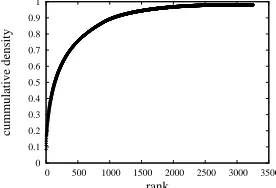
perform some exploratory data analysis. Figure 1 illustrates the 25th-most-frequent PMw history
con-text as a tree fragment. In the top-down model, the following elements have been generated:
• a parent nonterminal PP(IN/with) (a PP headed by the word with with the part-of-speech tagIN)
• the parent’s head childIN
• a right subcat bag containingNP-A(a single NP argument must be generated somewhere on the
0 0.1 0.2 0.3 0.4 0.5 0.6 0.7 0.8 0.9 1
0 500 1000 1500 2000 2500 3000 3500
cummulative density
rank
Figure 2: Cumulative density function for the PMw
history context illustrated in Figure 1. right side of the head child)
• a partially-lexicalized right-modifying nonter-minal
At this point in the process, a PMw parameter
condi-tioning on all of this context will be used to estimate the probability of the head word of theNP-A(NN), completing the lexicalization of that nonterminal. If a candidate head word was seen in training in this configuration, then it will be generated conditioning on the full context that crucially includes the head wordwith; otherwise, the model will back offto a history context that does not include the head word. In Figure 2, we plot the cumulative density func-tion of this history context. We note that of the 3258 words with non-zero probability in this con-text, 95% of the probability mass is covered by the 1596 most likely words.
[image:3.595.357.495.272.366.2]distribu-Back-off PM PMw
level ¯c d¯ n ¯c d¯ n
0 10.268 1.437 7.145 4.413 1.949 2.264
[image:4.595.161.454.71.133.2]1 558.047 3.643 153.2 60.19 8.454 7.120 2 1169.6 5.067 230.8 21132.1 370.6 57.02
Table 2: Average counts and diversities of histories of the PM and PMw parameter classes. c and d are
average history count and diversity, respectively. n= c
d is the average number of transitions from a history
context to some future.
1e-06 1e-05 0.0001 0.001 0.01 0.1
1 10 100 1000 10000
smoothed probability estimate
word frequency
(a) prob. vs. word freq., back-offlevel 1
1e-06 1e-05 0.0001 0.001 0.01 0.1
1 10 100 1000 10000 100000
smoothed probability estimate
word frequency
[image:4.595.118.492.216.340.2](b) prob. vs. word freq., back-offlevel 2
Figure 3: Probability versus word frequency for head words ofNP-A(NN)in thePPconstruction. tion of 3(a). 3(b) looks like a slightly “compressed”
version of 3(b) (in the vertical dimension), but the shape of the two distributions appears to be roughly the same. This observation will be confirmed and quantified by the experiments of §5.3
4 Entropies
A good measure of the discriminative efficacy of a parameter is its entropy. Table 3 shows the aver-age entropy of all distributions for each parameter class.4 By far the highest average entropy is for the PMw parameter class.
Having computed the entropy for every distri-bution in every parameter class, we can actually plot a “meta-distribution” of entropies for a pa-rameter class, as shown in Figure 4. As an ex-ample of one of the data points of Figure 4, con-sider the history context explored in the previous section. While it may be one of the most fre-quent, it also has the highest entropy at 9.141
3The astute reader will further note that the plots in Figure
3 both look bizarrely truncated with respect to low-frequency words. This is simply due to the fact that all words below a
fixed frequency are generated as the+UNKNOWN+word.
4The decoder makes use of two additional parameter classes
that jointly estimate the prior probability of a lexicalized non-terminal; however, these two parameter classes are not part of the generative model.
PH 0.2516 PT OPNT 2.517
PsubcatL 0.02342 PT OPw 2.853
PsubcatR 0.2147
PM 1.121
PMw 3.923
Table 3: Average entropies for each parameter class.
0 1 2 3 4 5 6 7 8 9 10
0 50000 100000 150000 200000 250000
entropy
rank
Figure 4: Entropy distribution for the PMw
parame-ters.
[image:4.595.342.509.405.466.2] [image:4.595.358.498.511.608.2]Back-off PM PMw
level min max avg median min max avg median
0 3.080E-10 4.351 1.128 0.931 4.655E-8 9.141 3.904 3.806
1 4.905E-7 4.254 0.910 0.667 2.531E-6 9.120 4.179 4.224
2 8.410E-4 3.501 0.754 0.520 0.002 8.517 3.182 2.451
[image:5.595.122.489.73.142.2]Overall 3.080E-10 4.351 1.121 0.917 4.655E-8 9.141 3.922 3.849
Table 4: Entropy distribution statistics for PM and PMw.
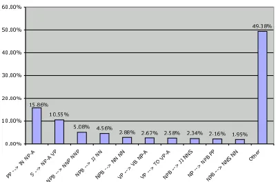
Figure 5: Total modifier word–generation entropy broken down by parent-head-modifier triple. distributions from PMw, 25 involve the
config-uration PP --> IN(IN/<prep>) NP-A(NN/. . .), where<prep>is some preposition whose tag isIN. Somewhat disturbingly, these are also some of the most frequent constructions.
To gauge roughly the importance of these high-frequency, high-entropy distributions, we per-formed the following analysis. Assume for the mo-ment that every word-generation decision is roughly independent from all others (this is clearly not true, given head-propagation). We can then compute the total entropy of word-generation decisions for the entire training corpus via
HPMw = X
c∈PMw
f (c)·H(c) (1)
where f (c) is the frequency of some history con-text c and H(c) is that concon-text’s entropy. The to-tal modifier word-generation entropy for the cor-pus with the independence assumption is 3,903,224 bits. Of these, the total entropy for contexts of the formPP → IN NP-Ais 618,640 bits, representing a sizable 15.9% of the total entropy, and the sin-gle largest percentage of total entropy of any parent-head-modifier triple (see Figure 5).
On the opposite end of the entropy spectrum, there are tens of thousands of PMw parameters
with extremely low entropies, mostly having to do with extremely low-diversity, low-entropy part-of-speech tags, such asDT,CC,INorWRB. Perhaps even
more interesting is the number of distributions with identical entropies: of the 206,234 distributions, there are only 92,065 unique entropy values. Dis-tributions with the same entropy are all candidates for removal from the model, because most of their probability mass resides in the back-offdistribution. Many of these distributions are low- or one-count history contexts, justifying the common practice of removing transitions whose history count is below a certain threshold. This practice could be made more rigorous by relying on distributional similarity. Fi-nally, we note that the most numerous low-entropy distributions (that are not trivial) involve generating right-modifier words of the head child of anSBAR
parent. The model is able to learn these construc-tions extremely well, as one might expect.
5 Distributional similarity and bilexical statistics
We now return to the issue of bilexical statis-tics. As alluded to earlier, Gildea (2001) per-formed an experiment with his partial reimplemen-tation of Collins’ Model 1 in which he removed the maximal-context back-off level from PMw, which
[image:5.595.85.285.191.323.2]performance, seemingly confirming the prevailing view.
But the 1.49% figure does not tell the whole story. The parser pursues many incorrect and ultimately low-scoring theories in its search (in this case, us-ing probabilistic CKY). So rather than askus-ing how many times the decoder makes use of bigram statis-tics on average, a better question is to ask how many times the decoder can use bigram statistics while pursuing the top-ranked theory. To answer this question, we used our parser to constrain-parse its own output. That is, having trained it on Sec-tions 02–21, we used it to parse Section 00 of the Penn Treebank (the canonical development test set) and then re-parse that section using its own highest-scoring trees (without lexicalization) as constraints, so that it only pursued theories consistent with those trees. As it happens, the number of times the de-coder was able to use bigram statistics shot up to 28.8% overall, with a rate of 22.4% for NPB con-stituents.
So, bigram statistics are getting used; in fact, they are getting used more than 19 times as often when pursuing the highest-scoring theory as when pursu-ing any theory on average. And yet there is no dis-puting the fact that their use has a surprisingly small effect on parsing performance. The exploratory data analysis of §3.3 suggests an explanation for this per-plexing behavior: the distributions that include the head word versus those that do not are so similar as to make almost no difference in terms of parse accuracy.
5.1 Distributional similarity
A useful metric for measuring distributional simi-larity, as explored by (Lee, 1999), is the Jensen-Shannon divergence (Lin, 1991):
JS (p kq )= 1 2
h
Dp
avgp,q
+Dq
avgp,q
i
(2) where D is the Kullback-Leibler divergence (Cover and Thomas, 1991) and where avgp,q =
1
2(p(A)+q(A)) for an event A in the event space of at least one of the two distributions. One inter-pretation for the Jensen-Shannon divergence due to Slonim et al. (2002) is that it is related to the log-likelihood that “the two sample distributions orig-inate by the most likely common source,” relating the quantity to the “two-sample problem”.
In our case, we have p = p(y|x1,x2) and q =
p(y|x1), where y is a possible future and x1,x2 are elements of a history context, with q representing a back-off distribution using less context. There-fore, whereas the standard JS formulation is
agnos-min max avg. median
JS0←1 2.729E-7 2.168 0.1148 0.09672 JS1←2 0.001318 1.962 0.6929 0.6986 JS0←2 0.001182 1.180 0.3774 0.3863
Table 5: Jensen-Shannon statistics for back-off pa-rameters in PMw.
tic with respect to its two distributions, and averages them in part to ensure that the quantity is defined over the entire space, we have the prior knowledge that one history context is a superset of the other, thathx1iis defined whereverhx1,x2iis. In this case, then, we have a simpler, “one-sided” definition for the Jensen-Shannon divergence, but generalized to the multiple distributions that include an extra his-tory component:
JS (p kq )=
X
x2
p(x2)·D (p(y|x1,x2) kp(y|x1) ) = Ex2D (p(y|x1,x2) kp(y|x1) ) (3)
An interpretation in our case is that this is the ex-pected number of bits x2 gives you when trying to predict y.5 If we allow x
2 to represent an arbitrary amount of context, then the Jensen-Shannon diver-gence JSb←a = JS (pb||pa) can be computed for
any two back-offlevels, where a,b are back-off
lev-els s.t. b < a (meaning pb is a distribution using
more context than pa). The actual value in bits of
the Jensen-Shannon divergence between two distri-butions should be considered in relation to the num-ber of bits of entropy of the more detailed distribu-tion; that is, JSb←ashould be considered relative to
H(pb). Having explored entropy in §4, we will now
look at some summary statistics for JS divergence. 5.2 Results
We computed the quantity in Equation 3 for every parameter in PMw that used maximal context
(con-tained a head word) and its associated parameter that did not contain the head word. The results are listed in Table 5. Note that, for this parameter class with a median entropy of 3.8 bits, we have a median JS divergence of only 0.097 bits. The distributions are so similar that the 28.8% of the time that the de-coder uses an estimate based on a bigram, it might as well be using one that does not include the head word.
5Or, following from Slonim et al.’s interpretation, this
quan-tity is the (negative of the) log-likelihood that all distributions
that include an x2 component come from a “common source”
≤40 words
§00 §23
Model LR LP LR LP
m3 n/a n/a 88.6 88.7
m2-emu 89.9 90.0 88.8 88.9
reduced 90.0 90.2 88.7 88.9
all sentences
Model §00 §23
m3 n/a n/a 88.0 88.3
m2-emu 88.8 89.0 88.2 88.3
[image:7.595.102.269.70.203.2]reduced 89.0 89.0 88.0 88.2
Table 6: Parsing results on Sections 00 and 23 with Collins’ Model 3, our emulation of Collins’ Model 2 and the reduced version at a threshold of 0.06. LR =labeled recall, LP=labeled precision.6
6 Distributional Similarity and Parameter Selection
The analysis of the previous two sections provides a window onto what types of parameters the pars-ing model is learnpars-ing most and least well, and onto what parameters carry more and less useful infor-mation. Having such a window holds the promise of discovering new parameter types or features that would lead to greater parsing accuracy; such is the scientific, or at least, the forward-minded research perspective.
From a much more purely engineering perspec-tive, one can also use the analysis of the previous two sections to identify individual parameters that carry little to no useful information and simply re-move them from the model. Specifically, if pb is
a particular distribution and pb+1 is its correspond-ing back-off distribution, then one can remove all parameters pbsuch that
JS (pb||pb+1)
H(pb)
<t,
where 0 < t < 1 is some threshold. Table 6 shows
the results of this experiment using a threshold of 0.06. To our knowledge, this is the first example
of detailed parameter selection in the context of a generative lexicalized statistical parsing model. The consequence is a significantly smaller model that performs with no loss of accuracy compared to the full model.6
Further insight is gained by looking at the per-centage of parameters removed from each parame-ter class. The results of (Bikel, 2004) suggested that the power of Collins-style parsing models did not
6None of the differences between the Model 2–emulation
results and the reduced model results is statistically significant.
PH 13.5% PT OPw 0.023%
PsubcatL 0.67% PM 10.1%
PsubcatR 1.8% PMw 29.4%
Table 7: Percentage of parameters removed from each parameter class for the 0.06-reduced model.
lie primarily with the use of bilexical dependencies as was once thought, but in lexico-structural depen-dencies, that is, predicting syntactic structures con-ditioning on head words. The percentages of Table 7 provide even more concrete evidence of this as-sertion, for whereas nearly a third of the PMw
pa-rameters were removed, a much smaller fraction of parameters were removed from the PsubcatL, PsubcatR
and PMclasses that generate structure conditioning
on head words. 7 Discussion
Examining the lower-entropy PMw distributions
re-vealed that, in many cases, the model was not so much learning how to disambiguate a given syn-tactic/lexical choice, but simply not having much to learn. For example, once a partially-lexicalized nonterminal has been generated whose tag is fairly specialized, such asIN, then the model has “painted itself into a lexical corner”, as it were (the extreme example isTO, a tag that can only be assigned to the word to). This is an example of the “label bias” problem, which has been the subject of recent dis-cussion (Lafferty et al., 2001; Klein and Manning, 2002). Of course, just because there is “label bias” does not necessarily mean there is a problem. If the decoder pursues a theory to a nonterminal/ part-of-speech tag preterminal that has an extremely low entropy distribution for possible head words, then there is certainly a chance that it will get “stuck” in a potentially bad theory. This is of particular concern when a head word—which the top-down model gen-erates at its highest point in the tree—influences an attachment decision. However, inspecting the low-entropy word-generation histories of PMw revealed
that almost all such cases are when the model is generating a preterminal, and are thus of little to no consequence vis-a-vis syntactic disambiguation. 8 Conclusion and Future Work
[image:7.595.339.512.71.108.2]in a parsing model, and follows up with a numerical analysis of properties of those distributions. In the course of this analysis, we have focused in on the question of bilexical dependencies. By constrain-parsing the parser’s own output, and by hypothe-sizing and testing for distributional similarity, we have presented evidence that finally explains that (a) bilexical statistics are actually getting used with great frequency in the parse theories that will ulti-mately have the highest score, but (b) the distribu-tions involving bilexical statistics are so similar to their back-off counterparts as to make them nearly indistinguishable insofar as making different parse decisions. Finally, our analysis has provided for the first time an effective way to do parameter selec-tion with a generative lexicalized statistical parsing model.
Of course, there is still much more analysis, hy-pothesizing, testing and extrapolation to be done. A thorough study of the highest-entropy distributions should reveal new ways in which to use grammar transforms or develop features to reduce the entropy and increase parse accuracy. A closer look at the low-entropy distributions may reveal additional re-ductions in the size of the model, and, perhaps, a way to incorporate hard constraints without disturb-ing the more ambiguous parts of the model more suited to machine learning than human engineering. 9 Acknowledgements
Thanks to Mitch Marcus, David Chiang and Ju-lia Hockenmaier for their helpful comments on this work. I would also like to thank Bob Moore for asking some insightful questions that helped prompt this line of research. Thanks also to Fernando Pereira, with whom I had invaluable discussions about distributional similarity. This work was sup-ported in part by DARPA grant N66001-00-1-9815. References
Daniel M. Bikel. 2002. Design of a multi-lingual, parallel-processing statistical parsing engine. In
Pro-ceedings of HLT2002, San Diego, CA.
Daniel M. Bikel. 2004. Intricacies of Collins’ parsing model. Computational Linguistics. To appear. E. Black, S. Abney, D. Flickenger, C. Gdaniec, R.
Gr-ishman, P. Harrison, D. Hindle, R. Ingria, F. Jelinek, J. Klavens, M. Liberman, M. Marcus, S. Roukos, B. Santorini, and T. Strzalkowski. 1991. A procedure for quantitatively comparing the syntactic coverage of English grammars. In Speech and Natural Language
Workshop, pages 306–311, Pacific Grove, California.
Morgan Kaufmann Publishers.
Ezra Black, Frederick Jelinek, John Lafferty, David Magerman, Robert Mercer, and Salim Roukos. 1992a. Towards history-based grammars: Using
richer models for probabilistic parsing. In
Proceed-ings of the 5th DARPA Speech and Natural Language Workshop, Harriman, New York.
Ezra Black, John Lafferty, and Salim Roukos. 1992b. Development and evaluation of a broad-coverage probabilistic grammar of english-language computer manuals. In Proceedings of the 30th ACL, pages 185– 192.
Eugene Charniak. 2000. A maximum entropy–inspired parser. In Proceedings of the 1st NAACL, pages 132– 139, Seattle, Washington, April 29 to May 4.
Michael John Collins. 1999. Head-Driven Statistical
Models for Natural Language Parsing. Ph.D. thesis,
University of Pennsylvania.
Michael Collins. 2000. Discriminative reranking for natural language parsing. In International Conference
on Machine Learning.
Thomas Cover and Joy A. Thomas. 1991. Elements of
Information Theory. John Wiley & Sons, Inc., New
York.
Jason Eisner. 1996. Three new probabilistic models for dependency parsing: An exploration. In
Proceed-ings of the 16th International Conference on Com-putational Linguistics (COLING-96), pages 340–345,
Copenhagen, August.
Jason Eisner. 2000. Bilexical grammars and their cubic-time parsing algorithms. In Harry Bunt and An-ton Nijholt, editors, Advances in Probabilistic and
Other Parsing Technologies, pages 29–62. Kluwer
Academic Publishers, October.
Daniel Gildea. 2001. Corpus variation and parser per-formance. In Proceedings of the 2001 Conference on
Empirical Methods in Natural Language Processing,
Pittsburgh, Pennsylvania.
Dan Klein and Christopher D. Manning. 2002. Condi-tional structure versus condiCondi-tional estimation in NLP models. In Proceedings of the 2002 Conference on
Empirical Methods for Natural Language Processing.
John Lafferty, Fernando Pereira, and Andrew McCal-lum. 2001. Conditional random fields: Probabilistic models for segmenting and labeling sequence data. In
ICML.
Lillian Lee. 1999. Measures of distributional similarity. In Proceedings of the 37th ACL, pages 25–32. Jianhua Lin. 1991. Divergence measures based on the
Shannon entropy. IEEE Transactions on Information
Theory, 37(1):145–151.
David Magerman. 1994. Natural Language Parsing as
Statistical Pattern Recognition. Ph.D. thesis,
Univer-sity of Pennsylvania, Philadelphia, Pennsylvania. Mitchell P. Marcus, Beatrice Santorini, and Mary Ann
Marcinkiewicz. 1993. Building a large annotated cor-pus of English: The Penn Treebank. Computational
Linguistics, 19:313–330.