Abstract— This paper proposes a population based adaptive tuning for dynamic position control of robot manipulators. The dynamic behavior of a robot manipulator is highly nonlinear, and the positional control is conventionally achieved by inverse dynamics feedforward and PID feedback controllers. The proposed method tunes the PID controller parameters using cross-entropy optimization to minimize the error in tracking a repeated desired trajectory in real-time. The stability of the system is granted by switching the inappropriate settings to a stable default using a real-time cost evaluation function.
The proposed tuning method is tested on a two-joint planar manipulator, and on a planar inverted pendulum. The test results indicated that the proposed method improves the settling time and reduces the position error over the repeated paths.
Index Terms— Cross entropy optimization, dynamic control,
PID tuning, population based optimization.
I. INTRODUCTION
Robot manipulators are mainly positioning devices with multiple degrees-of-freedom (DoF). Dynamic position control of robot manipulators is a well known problem in control engineering due to the multi-input-multi-output nonlinear behaviour of their equation of motion. There are a large number of excellent survey books and articles on the control of the manipulators [1]-[4]. In a typical position control problem, the plant is characterized by the dynamic equation of motion of the manipulator, which describes the motion of the joint displacements corresponding to the applied joint torques. The controller is designed to generate appropriate joint torques to track a desired task space trajectory, or equivalently to track the corresponding desired joint space trajectory. The conversion of trajectories from the task space to the joint space requires kinematic modeling of the robot manipulator. The equation of motion is obtained by one of the methods such as Newton-Euler, Lagrangian, and their backward and forward recursive applications.
The decentralized PD and PID control is the standard method for position control of the manipulator joint displacement. PD control can achieve global asymptotic stability in tracking a trajectory in the absence of gravity. The integral action of the PID control further compansates any
Manuscript received March 22, 2007.
Dr. M. Bodur is with the EMU- Computer Engineering Department, Mersin -10 Turkey. Phone: +90(533)876 4317; fax: +90(392)3650711; Submitted to ICCIS-07 for Evolutionary Systems topic. (e-mail: mehmet @ ieee . org ).
tracking offset due to gravitational forces [4]. Several methods were proposed in literature to obtain suitable propotional, integral and derivative controller gain settings: Kp, Ki and Kd. In absence of friction, the gains may be selected using a Lyapunov function candidate and LaSalle’s Invariance Principle [4]. Adaptive PID settings were also proposed for obtaining proper local gain settings based on plant identification and pole placement techniques [5].
Cross-Entropy (CE) Method is an information theoretic method of inference about an unknown probability density from a prior estimate of the density and new expected values [7]-[8]. CE Method was further developed as a combinatorial optimization method to obtain the optimal solutions for rare-event problems and optimization of the scalar functions [8]-[10]. Similar to Monte-Carlo and simulated annealing methods, it is one of the optimization methods with the proven convergence to the optimal parameters.
This paper is organized as follows: Section 2 presents the kinematics, dynamic modeling and control of a robot manipulator. Section 3 introduces the cross-entropy method for optimization of the controller gains. Section 4 explains the objective and algorithm of the optimization, Section 5 and 6 contains the experimental details and the results of the proposed parameter switching on a two-link planar manipulator, and on an inverted pendulum system. Section 7 concludes the paper.
II. KINEMATICSDYNAMICANDCONTROL The forward kinematics relation maps the joint space position q to the end-effector pose
p = f0(q) (1)
using homogenous link-frame coordinate transformation matrices. Denavit-Hartenberg (D-H) convention provides the D-H transformation matrix Ai that maps a coordinate at i-th frame to the (i−1)-st frame [11].
The Lagrangian method is a systematic method to obtain the equation of motion of a multi-degree-of-freedom open chain mechanism. The Lagrangian function L is defined by
L = K − P, where K is the kinetic energy, and P is the potential energy of the analyzed system. The partial derivatives of L
provide a simple means of calculation for the joint force and torques. The derivatives of the D-H transformation matrices Ai can be expressed by
i i
q
A
∂
∂
= QiAi , where Qi =
−
0 0 0 0
0 0 0 0
0 0 0 1
0 0 1 0
for revolute joints. (2)
An Adaptive Cross-EntropyTuning of the
PID Control for Robot Manipulators
This property provides a convenient form for the derivatives of the link transformation matrices 0Ti with respect to the j-th generalized-joint displacement variable qj .
Uij =
j i q
T
∂ ∂0
=
j i j q
A A A A
∂
∂( 1 2... ... )
= A1A2 ... QjAj ... Ai ; j ≤ i . (3) Linear or revolute, the kinetic energy of a mass dmi located at the position irdm and moving with the i-th coordinate frame is
d ki =12d mi0viT 0vi , (4)
where 0vi is the velocity of mass mi.
The total kinetic energy of the link requires the integration of
d ki over the complete mass of the i-th link.
ki =
∫
mi dki = 12Trace[(
Σ
ip=1Σ
r=i 1UipJpi UirTq˙rq˙p)]
, (5) where Jpi=∫mi irdmirdmTdmi is the pseudo-inertia matrix of the i-th link. The potential energy of i-th link due to the gravitational field is expressed using the mass mi, the center of mass icm and the gravitational acceleration vector gapi= − migaT 0Ti icm . (6)
Finally, the Lagrangian of the complete system is obtained
L= K−P =12
Σ
ni=1Σ
ik=1Σ
ir=1Trace(U
ikJpi UirT) q˙
r q˙p −Σ
n i=1mi gaT 0Tiicm (7) and its derivatives gives the generalized joint-force at the joint-j.τj = dt d
∂
∂
j
q L
& − qj
L ∂
∂
, (8)
τj =
Σ
i=jnΣ
k=n 1Trace(
UikJpiUijT)
q˙˙k +Σ
k=n 1Σ
r=n 1Trace(
UikrJpiUijT)
q ˙k q ˙r−
Σ
i=jn mi gaTUijicm . (9) Further, (8) and (9) can be organized to Uicker-Kahn form. τi =Σ
i=jn Dij˙˙qj +Σ
i=jnΣ
k=n 1Cijk q ˙j q ˙k +gi. (10) where Dij =Σni=j Trace(Uik JpiUijT) ; Cijk =Σ r=n 1Trace(UikrJpi UijT), and gj= − Σn
i=jmi gaTUijicm , are the inertial, coriolis, and gravitational terms of the equation of motion. The equation is also written in a matrix form [4]
τ = D(q) q˙˙ + C(q, q˙ ) q˙ + g(q) .
A constant field dc-motor converts the total control action by an almost linear relation of rotor current irotor to the joint torque τ = ki × irotor . Accordingly, without loss of generality, the torque coefficient ki is assumed ki=1 so that the joint torques are determined directly by the control action.
A fully actuated rigid manipulator has an independent control input for each degree-of-freedom, which simplifies its decentralized control. Robots with flexible links or joints have control problems and which may require singular perturbation and two-time-scale control techniques [4], [5].
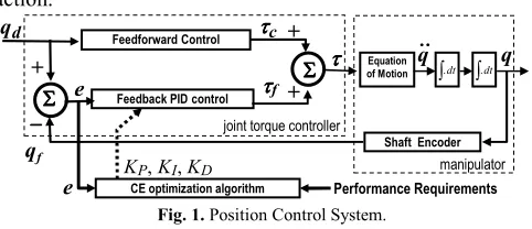
The equation of motion is highly nonlinear to apply independent PID control directly to each joint motion. The usual method is to apply the expected joint torques for the desired trajectory by a feedforward control, and correct any deviation from the trajectory by the feedback loop of the PID
control. The feedforward control action τc is obtained by the sum of the anticipated gravitational and inertial terms, so that all coriolis forces remains as a disturbance to the feedback loop
τc =Dc(qd) q˙˙d+gc(qd) ,
[image:2.612.316.557.186.290.2]where Dc and gc are the inertial coefficients and gravitational torques of the anticipated equation of motion; qd is the desired trajectory in joint space. The discrepancy of the anticipated equation of motion from the actual dynamics of the manipulator is expected to contribute to the disturbance torques, and thus a feedback control loop is inevitable for the stability of the control action.
Fig. 1. Position Control System.
The difference of the desired position qd(t) and the measured position qf (t) is called the displacement error e(t) of the control system. A proportional gain provides main correction of the error, an integral gain provides correction of the offset, and a derivative gain provides faster response of the controlled system.
τf = KPe(t) +KI
∫
tt0e(t) dt +KDe˙(t) . (13) Assuming that the anticipated feedforward control law can be predicted by the mechanical properties of the manipulator, the PID parameters remain to be determined for the optimum tracking of the specified joint space trajectory. The following section contains the cross entropy method, which is employed to find the optimum PID gains.III. CROSS ENTROPY METHOD
In the optimization of the PID gains, The closed loop control system is considered as a stochastic system with the controller parameters. Cross Entropy method is a population based optimization algorithm that utilize the scores of the trial runs optimal in the information rhetoric meaning.
Let X be the set of real valued states, and let the scores S be a real function on X. CE-method targets to find the minimum of S
over X, and the corresponding states x* satisfying the minimum γ* = S(x*) = minx∈X S(x), (14) by employing importance sampling and minimizing the cross entropy between the samples of a family of succeeding probability mass function f(-, vk). A naive random search can
find an expected value for x* and determine γ* with probability 1, if some of the scores S(x) for the random states x can satisfy the minimum. However, methods like Crude Monte-Carlo requires considerable computational effort because it uses homogeneously distributed random states in searching x*. CE method provides a methodology for creating a sequence of vectors x0, x1 ... and levels γ0, γ1, ... such that γ0, γ1, ...
converges to γ* and x0, x1 , ... converges to x*.
Equation of Motion
Shaft Encoder Σ
ΣΣ Σ
qf
qd
joint torque controller
Feedback PIDcontrol
e
ττττ FeedforwardControl
Σ ΣΣ Σ ττττc
ττττf
+
−−−−
+
+
CE optimization algorithm Performance Requirements
e
KP, KI, KD
q
∫.dt
q
manipulator ∫.dt
(11)
Define a collection of functions { H( - ; γ ) } on Χ, via
H( x ; γ ) = I{S(x(i)) >γ } ={1 if 0 if SS((xx) ≤ ) > γγ . (15)
for each x ∈ X, and threshold γ ∈ R. Let f(-; v) be a family of
probability mass function (pmf) on X, parameterized by a real valued vector v ∈ R. Consider the probability measure under
which the state x satisfies the threshold γ lv (γ) = Pv ( S(X) ≥ γ )
=
Σ
xH( x; γ ) f(-; v) = Ev H( X; γ ) , (16)where Ev denotes the corresponding expectation operator. It
converts the optimization problem to an associated stochastic rare event problem. Using the Importance Sampling (IS) simulation, the unbiased estimator of l with the random sets of states x(1), ... taken from different independent pmf f(x,v) and
g(x) is l^ = 1
N
Σ
Ni=1 I{S(x(i)) >γ }W (x(i)) , (17)
where W(x) = f(x,v)/g(x) is the likelihood ratio. Searching the
optimal importance sampling density g*(x) is problematic, since determination of g*(x) requires l to be known. Instead, the optimum tilting parameter v* of a pmf f(x, v) reduces the
problem to scalar case.
The tilting parameter v can be estimated by minimizing
Kullback-Leibler “distance” (also called cross entropy) between the two densities f(x) and g(x)
CE(f, g)=
∫
f(x) ln gf((xx) ) dx. (17) After reducing the problem to tilt parameter v, thecross-entropy between f (x, v) and the optimal distribution f(x, v*) is described by
CE(v, v*) := { } { }
≥ ≥
) , (
*) , (
ln ( )
) (
υ υ
γ γ
x f c
x f I
c I
Ea S X S X , (18)
where c =
∫
I{S(X)≥γ}f(x)dx . The optimal solution v* isobtained by solving v* from min
v CEN(
v) , where
CEN(v) =Ev1=N1
Σ
N i=1 I{S(x(i)) > γ }W (x(i), v, v*) , (19)For example, if all γ is equal to γ*, in that case lv(γ)=f(x*; γ),
which typically would be a very small number. lv(γ*) is
estimated by Importance Sampling with vk=v
v* = argmax
v¯ Σ
N
i=1 EvH(X; γ) ln f (X ; ¯v) , (20)
and using X(i), which are generated from pmf f (X ; v¯) by
argmax
v¯ Σ
N
i=1 H(X(i) ; γ) ln f (X(i) ; v¯) . (21)
However, the estimator of v* is only valid when H(X(i) ; γ) =1
for enough samples.
The CE-algorithm consist of the two phases: 1) Generate
random samples using f(-;vk), and calculate the estimate of the
objective function; 2) Update f(-;vk) on the basis of the data
collected in the first phase via the CE method. The main CE Algorithm is
1) Initialize k=0, and choose initial parameter vector v0=v.
2) Generate a sample of states x(1), ..., x(M) according to the
pmf f(-;vk) .
3) Calculate the scores S( x(i) ) for all i, and order them from
the biggest to the smallest,
s1, ≥ ... ≥sN .
Define γk = s[ρN] , where [ρN] is the integer part of ρN, so that
γk > γ, set γk = γ, this yields a reliable estimate by ensuring the
target event is temporarily made less rare for the next step if the target is not reached by at least a fraction of the samples.
4) For j=1, ..., 5, let
Σ
Mi=1I{S(x(i)) >γk }W (x(i) ; v , vk) x(ji)
vk+1,j=
Σ
Mi=1I{S(x(i)) >γk }W (x(i) ; v , vk)
. (22)
5) Increment k and repeat steps 2, to 5, until the parameter
vector has converged. Let v* denote the final parameter vector.
6) Generate a sample x(1), ..., x(N) according to the pmf
f(-; vk) and estimate l via the IS estimate
l^ = 1 N
Σ
N
i=1H (x(i)) W (x(i) ; v , v*) . (23)
Step (6) of the CE algorithm is not necessary in optimization of the scalar cost functions, since the goal is to minimize the cost rather than calculation of the probability of a rare event.
IV. OPTIMIZATION CRITERIA AND TEST METHOD
The optimization of motion control parameters of a manipulator using reinforcement, genetic, or other population methods comes across important problems in testing the generated parameter sets. These methods are mostly applied on simulations, because the unrestricted population may contain unstable controller settings, which may cause misoperation, and even damage of the robot system. Lin solved the problem by testing stability properties of the parameters before applying them to the dynamic control system [12]. His method is based on restricting the search space to a narrow region that guarantees Liapunov stability of the system.
Algorithm:
1) At initialization, specify a stable controller parameter set
ws, a real-time cost function J(t, p(t), pd(.) ), a cost threshold J*,
and a cost score function S( w, pd(.)). Initialize k=0, and j=1,
and choose initial vk = ws. Specify initial γk and 0<ρ<1, and so
that “the ratio of stable parameter vectors to all parameter
vectors” is higher than ρ. Τhis ensures reliable estimates of the
target. Select the coefficients 0 < α ≤ 1 and 0 < β ≤ 1 to update
vk+1 and γk+1 smoothly.
2) Generate a population of states w(1), ..., w(M) according to
the pmf f(γk;vk) .
3) For each w(i), at the beginning of a trajectory period pd(.)
switch the controller settings to w(i) , and during the period,
evaluate J(t, p, pd). Whenever J(t) exceeds J* switch the
controller settings to ws , so that system stays stable, and the
trajectory deviation remains within tolerable limits. At the
end of the trajectory period, calculate the cost score of the
sample, s(i)= S(w(i), pd).
4) Order the scores from the biggest to the smallest, i.e.,
s1, ≥ ... ≥sN .
Use γk = s[ρN] , where [ρN] is the integer part of ρN, to select the
elite subset of population. Estimate wk+1, and γk+1 from the
mean and standard deviation of the parameters in the elite subset. Update
wk+1 = αwk+1 + (1–α)wk,
βm = β - β (1− k 1) qs, and
γk+1 = βm γk+1,j + (1−β m) γk .
If vk+1converges to vk , increment j=j+1; else reset j=0.
5) Repeat the steps (2) – (4) until j=5, (i.e., the last 5
iterations converge to the target w*.)
The proposed method provides a higher degree of flexibility in specifying the cost function compared to many other controller parameter optimization techniques which are based on plant identification or state estimation techniques. For example, in the following simple demonstration, the cartesian
absolute path deviation ( e(t)= | p(t)−pd(.)| ) is used instead of
using the conventional trajectory tracking error (e(t)=
q(t)−qd(t) ) in joint space.
V. SIMPLE 2-LINK (2R)DEMONSTRATION
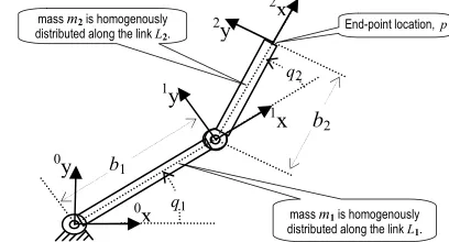
Consider the two link manipulator with two revolute joints
shown in Figure 1. The length of the links L1 and L2 are
respectively b1, and b2. The masses m1 and m2 are
homogenously distributed along the links L1 and L2. Coordinate
frames 0T, 1T and 2T are assigned for the base, L1, and L2 by
applying D-H convention as shown in Fig-1. The symbolic equation of motion for this planar manipulator is derived in symbolic toolbox of MATLAB using Lagrangian formulation
τ1=
(
13 m1b12+ 13m2b12 +m2b1b2 C2 +m2b12)
q..1+
(
13 m1b12−m1b1b2− 1
2 m1b12 C2+m1b22+m1b1b2C2
)
q ..2
− m2b1b2 S2 q.1q.2 − 12 m2b1b2 S2 q.2 2
+ 1
2 g
(
b1m1C1 + b2m2C12 +2 b1m2C1) ,
(24)τ2 = +
(
13m1b12−m1b1b2 − 12 m1b12C2+m1b22+m1b1b2C2)
q..1+ 1
3 m2b2
2q..2 + 1
2 m2 b1b2 S2q .
1 2 + 12 g m2b2C12 ,
(25)
where Ci, and Si, denote cos(qi) and sin(qi); Cij, and Sij, denote
cos(qi + qj) and sin(qi + qj).
[image:4.612.336.540.114.224.2]
Fig. 2. Parameters of the simulated manipulator with 2-revolute joints.
In the simulation, the equation of motion is integrated for m1 =
5 kg, m2 = 3 kg, b1 = 0.5 m and b2 = 0.4 m, reducing the
simulation model to
τ s,1 =
(
150 199+ 35 C2)
q..1 +(
1360 + 38 C2)
q..2−3 5 S2q
.
1q.2− 10 3 S2 q.2 2 + 12 g
(
112 C1+ 65 C12)
τ s,2 =
(
1360 + 38 C2)
q..1 + _425q..2 + 10 3S2 q.2 2 + 35 g C12. (26)All joint and actuator friction forces are assumed to be zero to prevent their stabilizing effect on the closed loop stability of the
system. The feedforward control force τc is calculated only from
the inertial and gravitational terms of a similar model (τc =
Dc(qd) q˙˙d+gc(qd) ) but with a higher load mass m2=3.5kg.
τ c,1 (q) =
(
600 887+ 10 7C2)
q..1+(
1360 + 38 C2)
q..2d +2 1g(
6C1+75C12)
τ c,2 (q) =
(
1360 + 38 C2)
q..1 + 10 7g C12 . (27)The test path is selected on a line segment in cartesian
workspace starting from the point (0x, 0y) = (0.2, 0) to the point
(0.7, 0.5) through the via-point (0.4, 0.2). The test trajectory is
calculated for ∆t = 1 ms intervals using parabolic blend with
linear segments trajectory generation method with via points [11] under the constraints: maximum linear velocity= 1m/s, and
linear acceleration 1 m/s2. The points of the desired trajectory
are shown in Fig. 2 for every 50 ms periods.
Stable control parameters were initialized to be ws=[K1P, K1I,
K1D K2P, K2I, K2D ] = [5000, 50, 100, 5000, 50, 100]; and cost
function was J(t, p(t), pd(t))= ||p(t), pd(t)|| which is the cartesian
distance of end-point position p(t) to the desired trajectory pd(t);
the cost threshold is J*= 0.002 m; the cost score function was
S( w, pd(.))=maxtJ(t) over one trajectory period; the standard
deviation of the gaussian pdf was γk = 0.5 ws ; population size
was N= 60; elite population ratio was ρ=0.05; smooth update
coefficients were α = 0.9 ; β = 0.9 ; and qs=5. The convergence
plot of cartesian tracking displacement error is shown in Fig. 5. The CE-optimization provided almost 50% reduction of cartesian displacement error. The oscillatory action of actuator torques may be prevented by assigning an additional cost on the derivative of the controller output.
b1
b2
0
x
0
y
1
x
1
y
q1
2
x
2
y
mass m1 is homogenously
distributed along the link L1.
mass m2 is homogenously
distributed along the link L2.
End-point location, p
0.1 0.2 0.3 0.4 0.5 0.6 0.7 0.8 0
0.1 0.2 0.3 0.4 0.5
0.8 0.9 1 1.1 1.2 1.3 1.4 1.5 -3
-2.5 -2 -1.5 -1 -0.5
(a) (b) (c)
Fig. 3. Plots of the desired trajectory (a) x vs. y (in meters), (b) q1 vs. q2 (in radians),
(c) the movement of the links in x-y plane.
Fig. 4. Convergence plot of the best-score for two-link manipulator.
VI. CONTROL OF AN INVERTED PENDULUM
The inverted pendulum is a well analyzed classical control problem [12], [13]. The objective is to track a desired cart
trajectory with a small deviation ex by applying an external
force f on the cart along x-axis while keeping the pendulum
stable in vertical position. The mechanical parameters of the system are introduced in Fig.6.
The equation of motion of the system is expressed by
[
mc+mp mpb Cqmpb Cq J+mpb2
] [
x& &
q& &
]
+[
Cc −mpbq&Sq
0 Cp
] [
x& q&]
+[
0
mpb gSq
]
=[
f
0
]
, (28)where Cq and Sq are cos(q) and sin(q), g is the acceleration
due to gravity, mc is the mass of cart, mp is the mass of the pole,
b is the half length of the pole, Cc is the friction coefficient of
cart, Cp is the friction of the pole, J is the mass moment of
inertial about the pole, and f is the force applied to the cart [12].
Two PID controllers were cascaded to reduce the tracking
errors ex = x – xd, and eq = q − qd, asymptotically to zero as
shown in Fig 7. Oscillatory behavior was expected since no predictive or inverse dynamic feedforward action employed. In the tests, the desired cart trajectory was specified by a square function switching between –0.01 and 0.01m with a period 25s.
Both the cart mass mc, and pole mass mp were selected 1 kg.,
and the half-length of the pole b was taken 2m.
[image:5.612.328.550.45.626.2]Fig. 6. Inverted Pendulum System.
Fig. 5 a. Tracking performance of manipulator with initial stable control parameter set ws.
`
Fig. 5 b. An unstable parameter set causes excessive cartesian error at t=0.42, and control is switched back to ws.
Fig. 5 c. The best parameter set reduced the cartesian error to 50%, but bounded oscillatory action of torques were observed
because of the high proportional gain.
Fig. 7. Block diagram of inverted pendulum system for parameter optimization
Equation of Motion
Shaft Encoder Σ
ΣΣ Σ
xd
cascaded controllers
PID
ex f x, q
Σ ΣΣ Σ
qd
qf
+
−−−− −−−−
+
CE optimization algorithm Performance Requirements
eq
KqP, KqI, KqD
PID
KxP, KxI, KxD
xf
x q
inverted pendulum
system
∫.dt ∫.dt
mc
f
x 0
mass
mp
q 2b
0 0.1 0.2 0.3 0.4 0.5 0.6 0
0.1 0.2 0.3 0.4 0.5
0.7
y
x
0 10 20 30 40 50 0.0012
0.0014 0.0016 0.0018 0.0020
best score
CE-iteration
0 0.5 1 1.5 2 2.5
-40 -20 0 20 40
60error along x and joint-1 KP=5000 5000 KI=200 200 KD=80 80
time (s) : (pd-ps)x10000
: (qd-qs)x10000 : Torque (N.m)
0 0.5 1 1.5 2 2.5
-40 -20 0 20
40 error along y and joint-2 : (pd-ps)x10000 : (qd-qs)x10000 : Torque (N.m)
time (s)
0 0.5 1 1.5 2 2.5
0 10 20
30 maximum deviation from the path
: cart-dev x10000 (m) : switchback 0:off 1:on
time
0 0.5 1 1.5 2 2.5
-50 0 50
error along x and joint-1 KP=3132 2121 KI=268 221 KD=50 98
time (s) : (pd-ps)x10000
: (qd-qs)x10000
0 0.5 1 1.5 2 2.5
-50 0
50 error along y and joint-2
: (pd-ps)x10000 : (qd-qs)x10000 : Torque (N.m)
time (s)
0 0.5 1 1.5 2 2.5
0 20 40
60maximum deviation from the path
: cart-dev x10000 (m) : switchback 0:off 1:on
time
100 : Torque (N.m)
0 0.5 1 1.5 2 2.5
-20 0 20 40
60error along x and joint-1 KP=13032 5391 KI=452 46 KD=136 161
time (s) : (pd-ps)x10000
: (qd-qs)x10000 : Torque (N.m)
0 0.5 1 1.5 2 2.5
-40 -20 0 20
40error along y and joint-2
: (pd-ps)x10000: (qd-qs)x10000 : Torque (N.m)
time (s)
0 0.5 1 1.5 2 2.5
0 5 10
15maximum deviation from the path : cart-dev x10000 (m) : switchback 0:off 1:on
time q1
q2 y
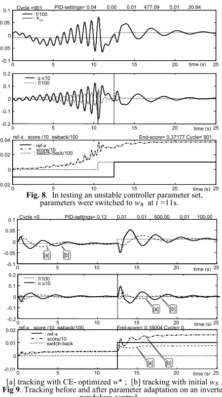
[image:5.612.49.298.51.237.2] [image:5.612.124.234.563.677.2]Fig. 8. In testing an unstable controller parameter set, parameters were switched to ws at t =11s.
[a] tracking with CE- optimized w* ; [b] tracking with initial ws .
Fig 9. Tracking before and after parameter adaptation on an inverted pendulum control.
The pole inertia Jp was taken 16/3. The friction coefficients
on the cart Cc, and on the pole Cp were taken 0.01, and the
gravitational acceleration was assumed 9.8 m/s2. Equation of
motion was integrated over ∆ t=5ms time steps using
trapezoidal method. Initially, the inverted pendulum was
stabilized by the control parameter set ws =[KxP, KxI, KxD,KqP,
KqI, KqD] = [0.13 0.01 0.01 500 0.01 100 ]. The cost function
was specified using the quadratic displacement errors ex2, eq2,
and their integrals:
S(w(i), pd, t) =20 ex2 + 30 ∫ex2dt + 50 eq2 + 100 ∫eq2 dt. (29)
For each w(i), the parameter set was switched at the beginning of
the desired trajectory cycle, for 50s. The value of S(w(i), pd, t) at
the end of the trajectory cycle was used for the score s(i).
Control parameters were switched back to the stable parameter
set ws at the threshold of S(w(i), pd) > 0.3. For the CE method,
the initial standard deviation of the gaussian pdf was selected
γk = 0.5 ws; population size was N = 60; elite population ratio
was ρ = 0.05; smooth update coefficients were selected to be α = 0.9, β = 0.9 , and qs = 5.
The plot of x and q for the initial stable parameter set, and for
the cost optimized parameter set is shown in Fig. 5, and a typical control parameter switching due to unstable character of the
tested parameter set w(i) is plotted in Fig. 8. The initial and final
performance of the cart and pole system is shown in Fig. 9.
VII. CONCLUSION
This study proposes a real time evolutionary search method that provides stability by switching the unstable control parameters with a prespecified stable parameter set whenever a tracking error based cost function exceeds a threshold. The proposed method has been tested successfully on two cases, on an open chain manipulator dynamic control, and on the control of an inverted pendulum. The second problem is relatively difficult since without a feedforward or predictive control the system is stable only in a very narrow band of PID parameter settings.
During the tests none of these two systems has been fallen into non controllable states. Even though some of the oscillatory controller settings collected better scores than similar but less oscillatory settings, the mean of the elites always remained preferably stable. In both cases, a considerable reduction of the specified cost function reaching up to 50% is achieved by cross-entropy optimization method during the progress of its repetitive operation.
ACKNOWLEDGMENT
Special thanks go to my colleague Dr. Adnan Acan for discussing several issues on implementation of the proposed method. Thanks to the graduate robotic course students: Maneli Badakshan, Vassilya Abdulova, Dilek Beyaz, Duygu Çelik for their efforts in reproduction of the trajectory planning algorithms; M. Reza Najiminaini, and A. A. Abed for their efforst in deriving the symbolic equation of motion.
REFERENCES
[1] Paul, R.C., “Modeling, Trajectory Calculation, and Servoing of a Computer Controlled Arm” Stanford A.I. Lab, A.I. Memo 177, Stanford, CA, Nov.1972.
[2] Paul, R.P., Robot Manipulators: Mathematics Programming, and
Control, MIT Press. Cambridge 1982.
[3] Fu, K.S., Gonzales, R.C., Lee C.S.G., Robotics Control, Sensing, Vision, and Intelligence, Mc.Graw-Hill International Ed. Singapore, 1988. [4] Mark W. Spong", "Motion Control of Robot Manipulators", online
article: url:citeseer.ist.psu.edu/165889.html.
[5] Bodur M., Sezer M. E., Adaptive control of flexible multilink manipulators, Int.J.Control, vol.58, no.3, pp 519-536, 1993.
[6] Rubinstein, R. Y. and Kroese, D.P. (2004). The Cross-Entropy Method:A
Unified Approach to Combinatorial Optimization, Monte-Carlo Simulation and Machine Learning. Springer-Verlag, New York. [7] Kullback S. Information theory and statistics. NY: Wiley, 1959. [8] J. Shore and R. Johnson. Properties of cross-entropy minimization. IEEE
Trans. Information Theory, 27(4):472-482, 1981
[9] D.P. Kroese and K.-P. Hui: Applications of the Cross-Entropy Method in Reliability, Computational Intelligence in Reliability Engineering (SCI) 40, 37–82 Springer-Verlag Berlin Heidelberg (2007).
[10] P.T. de Boer, D.P. Kroese, S. Mannor, and R.Y. Rubinstein. A tutorial on the cross-entropy method. Annals of Operations Research, 2004 [11] Uicker, J. J., Denavit, J. , Hartenberg, R. S., An iterative method for the
displacement analysis of spatial mechanisms. Journal of Applied Mechanics. 26. 309-314, 1964.
[12] S. B. Niku, Introduction to Robotics, Analysis, Systems, Applications. Prentice Hall Inc. pp 153-165, 2001.
[13] Chuan-Kai Lin, Reinforcement learning adaptive fuzzy controller for robots, Fuzzy Sets and Systems, Elsevier Vol.137, pp.339-352, 2002. [14] Shozo Mori, et al., Control of unstable mechanical system, control of
pendulum, Internat. J. Control 23 (5) pp. 673–692, 1976
-0.1 -0.05 0 0.05 0.1
0 5 10 15 20 25
Cycle =0 PID-settings= 0.13 0.01 0.01 500.00 0.01 100.00
: f/100
time (s)
-0.2 -0.1 0 0.1 0.2
0 5 10 15 20 25
: q x10
time (s)
-0.01 0 0.01 0.02
0 5 10 15 20 25
ref-x score /10 swback/100 End-score= 0.16004 Cycle= 0
time (s) : ref-x
: score/10 : switch-back
[a] [b]
[a] [b]
[b] [a]
0 5 10 15 20 25
-0.1 -0.05 0 0.05
0.1 Cycle =901 PID-settings= 0.04 0.00 0.01 477.09 0.01 20.84 : x
ref : f/100
time (s)
0 5 10 15 20 25
-0.2 -0.1 0 0.1 0.2
: q x10 : f/100
time (s)
0 5 10 15 20 25
-0.02 0 0.02
0.04ref-x score /10 swback/100 End-score= 0.37177 Cycle= 901
time (s) : ref-x
[image:6.612.65.284.44.436.2]