Graph-Based Collective Lexical Selection
for Statistical Machine Translation
Jinsong Su1,2, Deyi Xiong3∗, Shujian Huang2, Xianpei Han4, Junfeng Yao1 Xiamen University, Xiamen, P.R. China1
State Key Laboratory for Novel Software Technology, Nanjing University, P.R. China2 Soochow University, Suzhou, P.R. China3
Institute of Software, Chinese Academy of Sciences, Beijing, P.R. China4
{jssu, yao0010}@xmu.edu.cn [email protected] [email protected] [email protected]
Abstract
Lexical selection is of great importance to statistical machine translation. In this paper, we propose a graph-based frame-work for collective lexical selection. The framework is established on atranslation graphthat captures not only local associ-ations between source-side content words and their target translations but also target-side global dependencies in terms of relat-edness among target items. We also in-troduce a random walk style algorithm to collectively identify translations of source-side content words that are strongly related in translation graph. We validate the ef-fectiveness of our lexical selection frame-work on Chinese-English translation. Ex-periment results with large-scale training data show that our approach significantly improves lexical selection.
1 Introduction
Lexical selection, which selects appropriate trans-lations for lexical items on the source side, is a cru-cial task in statistical machine translation (SMT). The task is closely related to two factors: 1) asso-ciations of selected translations with lexical items on the source side, including corresponding source items and their neighboring words, and 2) depen-dencies1 between selected target translations and
other items on the target side.
As translation rules and widely-used n-gram language models can only capture local associ-ations and dependencies, we have witnessed
in-∗Corresponding author.
1Please note that dependencies in this paper are not nec-essarily syntactic dependencies.
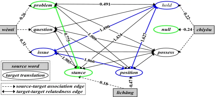
creasing efforts that attempt to incorporate non-local associations/dependencies into lexical selec-tion. Efforts using source-side associations mainly focus on the exploitation of either sentence-level context (Chan et al., 2007; Carpuat and Wu, 2007; Hasan et al., 2008; Mauser et al., 2009; He et al., 2008; Shen et al., 2009) or the utilization of document-level context (Xiao et al., 2011; Ture et al., 2012; Xiao et al., 2012; Xiong et al., 2013). In contrast, target-side dependencies attract little attention, although they have an important im-pact on the accuracy of lexical selection. The most common practice is to use language mod-els to estimate the strength of target-side depen-dencies (Koehn et al., 2003; Shen et al., 2008; Xiong et al., 2011). However, conventional n-gram language models are not good at capturing long-distance dependencies. Consider the exam-ple shown in Figure 1. As the translations of pol-ysemous words “w`ent´ı”, “ch´ıyˇou” and “l`ıchˇang” are far from each other, our baseline can only correctly translate “l`ıchˇang” as “stance”. It in-appropriately translates the other two words as “problem” and null, respectively, even with the support of an n-gram language model. If we could model long-distance dependencies among target translations of source words “w`ent´ı”(issue), “ch´ıyˇou”(hold) and “l`ıchˇang”(stance), these trans-lation errors could be avoided.
In order to model target-side global dependen-cies, we propose a novel graph-based collective lexical selection framework for SMT. Specifically,
• First, we propose a translation graph to model not only local associations between source-side content words and their target trans-lations but also global relatedness among target-side items.
wèntí= {problem, question, issue ...}
chíyŏu= {hold, null, possess ...}
lìchăng= {stance, position ...}
Tran: For this problem , two sides of the same or similar stance . Ref: Both sides hold the same or similar position on this issue .
Src:对于/P这/DT问题/NN,/PU双方/PN持有/VV相同/VA的/DEG立场/NN
[image:2.595.137.465.64.185.2]duìyú zhè wèntí , shuāngfāng chíyŏu xiāngtóng de lìchăng
Figure 1: A Chinese-English translation example to illustrate the importance of target-side long-distance dependencies for lex-ical selection. Dotted lines show long-distance dependencies of source content words. Three content words “w`ent´ı”, “ch´ıyˇou”, “l`ıchˇang”, and their candidate translations with high translation probabilities are also presented.Src: A Chinese sentence with part-of-speech tags.Tran: system output.Ref: reference translation.
• Second, we introduce a collective lexical se-lection algorithm, which can jointly identify translations of all source-side content words in the translation graph.
• Finally, we incorporate confidence scores of candidate translations in the translation graph, which are derived by the collective se-lection algorithm, into SMT to improve lexi-cal selection.
We validate the effectiveness of our graph-based lexical selection framework on a hierarchi-cal phrase-based system (Chiang, 2007). Exper-iment results on the NIST Chinese-English test sets show that our approach significantly improves translation quality.
We begin in Section 2 with the construction of translation graph for each translated sentence. Then, we propose a graph-based collective lexical selection framework for SMT in Section 3. Ex-periment results are reported in Section 4. We summarize and compare related work in Section 5. Finally, Section 6 presents conclusions and di-rections for future research.
2 Translation Graph
Formally, a translation graph is a weighted graph
G=(N, E). In the node set N, each node repre-sents either a source word or a target translation that contains one or multiple target words. In the edge setE, an edge linking a source word to a tar-get translation is referred to as asource-target as-sociation edge, and an edge connecting two target translations is called as atarget-target relatedness edge. In Section 2.1 and 2.2, we will answer the following two questions on the translation graph:
• Which source words and their translations should be included in the translation graph?
• How can we measure the strength of the above two types of relations in the graph with edge weights?
2.1 Graph Nodes
For a source sentence, the most ideal translation graph is a graph that includes all source words and their candidate translations. However, this ideal graph has two problems: intensive compu-tation for graph inference and difficulty in mod-eling dependencies between function and content words. In order to get around these two issues, we only consider lexical selection for source content words2.
We first identify source-side content word pairs using statistical metrics, and then keep word pairs with a high relatedness strength in the translation graph. To be specific, we use pointwise mutual in-formation (PMI) (Church and Hanks, 1990) and co-occurrence frequency to measure the related-ness strength of two source-side words s and s0
position
hold
null
possess problem
question
issue
0.22
0.18
0.24 0.491
0.31 0.26
stance
0.
47
1.985
1.43 4 1.490
1.62 7
1.866
0.7 75
chíyŏu wèntí
1.009
lìchăng source word
target translation
[image:3.595.128.475.62.218.2]source-target association edge target-target relatedness edge
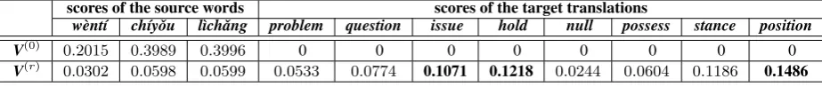
Figure 2: Translation graph of the example shown in Figure 1. Relatedness scores on edges are shown for two group of translations{“problem”, null, “stance”}(green) and{“issue”, “hold”, “position”}(blue), which are estimated with PMI. Note that thenullnode does not have any relations with other nodes. Besides, two translation combinations{“problem”,null, “stance”}(green) and{“issue”, “hold”, “position”}(blue) have different strengths of relatedness.
jective. For example, in the Chinese sentence in Figure 1, the adjective “xi¯angt´ong” is only related to the noun “l`ıchˇang” although it also frequently co-occur with “w`ent´ı”.
After identifying source-side content word pairs, we collect all target translations of these content words from extracted bilingual rules ac-cording to word alignments. These content words and target translations are used to build a transla-tion graph, where each node represents a source-side content word or a candidate target transla-tion. Note that there may be hundreds of differ-ent translations for a source word. For simplicity, we only consider target translations from transla-tion optransla-tions that are adopted by the decoder after rule filtering. Let’s revisit the example in Figure 2, we include the following target translations in the translation graph: “problem”, “question”, “issue”, “hold”,null, “possess”, “stance” and “position”.
2.2 Edges and Weights
In this section, we introduce how we calculate weights for two kinds of edges in a translation graph.
2.2.1 Source-Target Association Edge
Connecting a source-side content word and its candidate target translations, a source-target asso-ciation edge provides a way to propagate transla-tion associatransla-tion evidence from a source word to its candidate translations. Obviously, the stronger the association between a source word and its can-didate translation, the more evidence the corre-sponding edge will propagate. For each source-side content word, we obtain its candidate
trans-lations via the kept word alignments. Following Xiong et al. (2014), we allow a target translation to be either a phrase of length up to 3 words or
nullwhensis not aligned to any word in the cor-responding bilingual rule. We define the weight of the edge from a source-side content wordsto its target translation˜tas follows:
W eight(s→˜t) =P T P(s,˜t) ˜
t0∈N(s)T P(s,˜t0) (1)
where N(s) denotes the set of candidate target translations of s kept on the translation graph, and T P(s,˜t) measures the probability of s be-ing translated to ˜t. It is very important to note that there is no evidence propagated from a target translation to a source word, as source-target asso-ciation edges only go from a source-side content word to its translations.
We computeT P(s,˜t)according to the principle of maximal likelihood as follows:
T P(s,˜t) = countcount(s,(st˜)) (2)
wherecount(s,˜t)indicates how oftensis aligned to ˜t in the training corpus. Using this method, we can compute the translation probabilities of thesource-target association edgesin Figure 2 as follows: TP(“w`ent´ı”, “issue”)=0.31,TP(“ch´ıyˇou”, “hold”)=0.22 andTP(“l`ıchˇang”, “position”)=0.47.
2.2.2 Target-Target Relatedness Edge
dependencies between translations of any two dif-ferent source words.
Computing the weight of a target-target related-ness edge is crucial for our method. Intuitively, the stronger co-occurrence strength two transla-tions have, the more evidence should be propa-gated between them. Therefore we calculate the weight of a target-target related edge based on the co-occurrence strength of two translations linked by the edge. Formally, given the translationt˜of source-side content word sand the translation t˜0
of source-side content words0, the weight of the
edge from˜tto˜t0is defined as follows:
W eight(˜t→t˜0)=P RS(˜t,˜t0) ˜
t00∈N(˜t)RS(˜t,˜t00) (3)
where N(˜t) denotes the set of candidate transla-tions that link to ˜t, and RS(˜t,˜t0) measures the
strength of relatedness between˜t and˜t0 which is
calculated as the average word-level relatedness over all content words in these two translationst˜
and˜t0.
As for the word-level relatednessRS(t, t0)for
a content word pair (t, t0), we estimate it with
the following two approaches over collected co-occurring word pairs within a window of sizedt: (1)RS(t, t0)is computed as a bigram conditional
probabilityplm(t0|t) via the language model; (2) Following (Xiong et al., 2011) and (Liu et al., 2014), we employ PMI to define RS(t, t0) as
lnp(t)p(tp(t,t0)0).
3 Collective Lexical Selection Algorithm Based on the translation graph, we propose a col-lective lexical selection algorithm to jointly iden-tify translations of all source words in the graph.
3.1 Problem Statement and Solution Method
As stated previously, the translation of a source-side content wordsshould be: 1) associated with
s; 2) related to the translations of other source-side content words. Thus, in the translation graph, the translation ofsshould be a target-side node which has: 1) an association edge with the node of s; 2) many relatedness edges with other target-side nodes that represent translations of other source words.
Let’s revisit Figure 2. If we know that the trans-lation of “w`ent´ı” is “issue”, the relatedness be-tween (“issue”, “hold”) and between (“issue”,
“position”) can provide evidences that “hold” and “position” are the correct translations of “ch´ıyˇou” and “l`ıchˇang”, respectively. On the other hand, the candidate translation “problem” is less related to “hold” and “position”, which may suggest that it is not likely to be the correct translation of “w`ent´ı”, even if it has a strong source-target as-sociation relation with “w`ent´ı”. However, in the translation graph, the correct target translation of a source word depends on correct translations of other source words in the graph, and vice versa. So how do we find these correct translations?
We propose aRandom Walk(Gobel and Jagers, 1974) style algorithm to solve this problem, aim-ing to use both local source-target associations and global target-target relatedness simultane-ously during translation. In our algorithm, we as-sign each node an evidence score in the transla-tion graph, which indicates either the importance of a source word (for a source word node) or the confidence of a target translation being a correct translation (for a target word node). Specifically, we perform collective inference on the translation graph as follows:
• First, we set initial evidence scores for nodes in the translation graph.
• Second, evidence scores are simultaneously updated by propagating evidences along edges in the translation graph.
In the following sub-section, we describe the two steps in detail.
3.2 Details of Our Algorithm
Using the algorithm shown in Algorithm 1, we iteratively derive evidence scores for candidate translations.
3.2.1 Notations
For a translation graph with n nodes, we assign each node an index from 1 tonand use this index to represent the node. We also use the following two notations:
• The evidence vector V: an n-dimensional vector where theith componentViis the ev-idence score contained in this node (if node
Algorithm 1Collective Inference in Translation Graph. Input: S: the set of source-side content words, andS(i)
denotes the source word of nodei; k: the number of source-side content words ;
T: the set of all candidate target translations, andT(j)
denotes the target translation of nodej; l: the number of candidate target translations;
λ: the reallocation weight;
maxIter: the maximum iteration number;
: the difference threshold; 1: fori= 1,2...,k
2: forj= 1,2...,l
3: if S(i)is linked toT(j)
4: Mk+j,i←Weight(S(i)→T(j))
5: forj1= 1,2...,l 6: forj2= 1,2...,l
7: if T(j1)is linked toT(j2)
8: Mk+j2,k+j1→Weight(T(j1)→T(j2)) 9: fori= 1,2...,k
10: V(0)
i ←Importance(S(i))
11: forj= 1,2...,l 12: V(0)
k+j←0
13: δ← ∞ 14: r←1
15: while r≤maxIter && δ > do
16: V(r)←(1−λ)×M×V(r−1)+λ×V(0)
17: δ← kV(r)−V(r−1)k 2
18: r←r+ 1
19: end while 20: fori= 1,2...,k 21: forj= 1,2...,l
22: ifS(i)is linked toT(j)
23: LexiTable(S(i),T(j))←normalize(V(r) k+j)
Return: LexiTable;
evidence vector, andV(r)to represent the ev-idence vector we obtain at therth iteration.
• The evidence propagation matrix M: an
n×nmatrix whereMij is the evidence prop-agation ratio from nodej to node i, and its value is the weight of the edge from nodej
to nodei.
3.2.2 Algorithm
In Algorithm 1, we jointly infer the evidence scores of all candidate translations in the follow-ing three steps.
In Step 1, we calculate the evidence propaga-tion matrixMaccording to the method described in Section 2.2 (equations (1) and (3)) (Lines 1-8). InStep 2, we adopt different methods to set the value of V(0) according to the node type. If the node corresponds to a source word, we set the ini-tial value using its importance score in the
trans-lation graph, as implemented in (Han et al. 2011) (Lines 9-10). We calculate the importance score of the source wordsusingtf.idf as follows:
Importance(s) = P tf.idf(s)
s0∈Nsrctf.idf(s0) (4)
whereNsrcis the set of source words in the trans-lation graph. If the node corresponds to a target translation, its initial evidence score is 0 (Lines 11-12).
In Step 3, evidences are simultaneously rein-forced by propagating them among semantically related translations (Lines 13-19). Specific to our algorithm, we update them by propagating evi-dences according to different types of relations in the evidence propagation matrixM. Formally, the recursive update of the evidence vector is defined as follows:
V(r)=M×V(r−1) (5)
whereris the number of iterations.
One problem with the above equation is that some nodes in the translation graph do not have evidence outgoing edges, such as translation nodes containing only function words or thenull node. The evidence will disappear when passing through these nodes. To solve this problem, we propagate evidence in the form of reallocation: we reallocate a fraction of evidence to the initial evidence vector
V(0)at each step. The new recursive update of the evidence vector is formulated as follows:
V(r)= (1−λ)×M×V(r−1)+λ×V(0) (6)
whereλ∈(0,1)is the fraction of the reallocated evidence. We keep updating the evidence vec-tor according to this equation (Line 16), until the maximal number of iterationmaxIteris reached or the Euclidean distance (Line 17) between evi-dence vectors calculated in two consecutive itera-tions is less than a pre-defined threshold (Line 15).
In this way, we jointly infer the evidence scores of all candidate target translations in the transla-tion graph. Table 1 gives the evidence scores of the example in Figure 2. We can find that our sys-tem enhanced with target translation dependencies is able to select correct translations.
3.2.3 Integration of Derived Evidence Score
scores of the source words scores of the target translations
w`ent´ı ch´ıyˇou l`ıchˇang problem question issue hold null possess stance position
V(0) 0.2015 0.3989 0.3996 0 0 0 0 0 0 0 0
[image:6.595.73.535.63.112.2]V(r) 0.0302 0.0598 0.0599 0.0533 0.0774 0.1071 0.1218 0.0244 0.0604 0.1186 0.1486
Table 1: The initial and final evidence scores of some source words and their target translations in Figure 2. Here we set the reallocation weightλas 0.15. Note that the translations “issue”, “hold” and “position” are given high evidence scores.
we infer evidence scores of translations repre-sented by graph nodes using the above-mentioned algorithm before decoding. Then, for each can-didate translation of a source-side content word, we normalize its evidence score over the cor-responding translation graph to form an addi-tional lexical translation probability (Lines 20-23). For instance, the normalized evidence score of “ch´ıyˇou” translated into “hold” is calculated as 0.1218/(0.1218 + 0.0244 + 0.0604)≈0.5895. In this way, for each bilingual rule with word align-ments, we will obtain a new lexical weight which can be used together with the original translation probabilities and lexical weight to improve lexical selection in SMT.
4 Experiments 4.1 Setup
Our bilingual training corpus is the combina-tion of the FBIS corpus and Hansards part of LDC2004T07 corpus (1M parallel sentences, 54.6K documents, with 25.2M Chinese words and29M English words). We word-aligned them usingGIZA++(Och and Ney, 2003) with the op-tion “grow-diag-final-and”. We chose the NIST evaluation set of 2005 (MT05) as the development set, and the sets of MT06/MT08 as test sets. We used SRILM Toolkit (Stolcke, 2002) to train one 5-gram language model on the Xinhua portion of Gigaword corpus.
To construct translation graphs, we first used the
ZPar toolkit3 and the Stanford toolkit4 to
prepro-cess (word segmentation, PoS tagging and so on) Chinese and English sentences, respectively. We used the Chinese part of our bilingual corpus and an additional Chinese LDC Xinhua news corpus (10.2M sentences with 279.9M words) as train-ing data to collect Chinese word pairs. We set window size ds=15, thresholds pmi=0, cf=5 to identify Chinese related word pairs in the NIST translated sentences. Averagely, these three sets contain 13.5, 10.3 and 9.5 content words used
3http://people.sutd.edu.sg/∼yue zhang/doc/index.html 4http://nlp.stanford.edu/software
to build translation graphs per sentence, respec-tively. Using the English part of our bilingual cor-pus and the Xinhua portion of Gigaword corcor-pus as training data, we set window size dt=20, and used the SRILM toolkit with Witten-Bell smooth-ing and PMI to calculate relatedness strengths for target-side translations. To avoid data sparseness, we build the graph using the surface forms of words while calculating the word relatedness at the lemma level. To achieve this, we converted each word into its corresponding lemma with the exception of adjectives and adverbs. In the proce-dure of collective lexical selection, the difference thresholdwas set as10−10, and the maximal it-eration numbermaxIter100.
We reimplemented the decoder of Hiero (Chi-ang, 2007), a famous hierarchical phrase-based (HPB) system. HPB system is a formally syntax-based system and delivers good performance in various translation evaluations. During decod-ing, we set thettable-limitas20, thestack-sizeas 100. The translation quality is evaluated by case-insensitive BLEU-4 metric (Papineni et al., 2002). To alleviate the impact of the instability of MERT (Och, 2003), we ran it three times for each exper-iment and reported the average BLEU scores as suggested in (Clark et al., 2011). Finally, we con-ductedpaired bootstrap sampling (Koehn, 2004) to test the significance in BLEU score differences.
4.2 Our Method vs Other Methods
In the first group of experiments, we investigated the effectiveness of our model by comparing it against the baseline as well as two additional mod-els: (1) lexicalized rule selection model (He et al., 2008) (LRSM), which employs local context to improve rule selection in the HPB system; (2)
topic similarity model(Xiao et al., 2012)5(TSM),
which explores document-level topic information for translation rule selection in the HPB system. Furthermore, we combined our model with the two models to see if we could obtain further im-provements. For this, we integrated the new
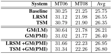
System MT06 MT08 Avg Baseline 30.25 21.25 25.75
LRSM 31.12 21.98 26.55
TSM 30.79 21.90 26.35
GM(LM) 30.64 21.78 26.21
GM(PMI) 31.02 21.77 26.40
LRSM +GM(PMI) 31.66 22.23 26.95
[image:7.595.85.278.61.154.2]TSM +GM(PMI) 31.34 22.26 26.80
Table 2: Experiment results on the test sets withλ=0.15.Avg = average BLEU scores,GM(LM)andGM(PMI)denote our model using the measure based on language model and PMI, respectively.
cal weight learned by our model as a new feature into theLRSM/TSMsystem.
Table 2 reports the results. All models outper-form the baseline. Especially, our graph-based lexical selection model GM(PMI) achieves an av-erage BLEU score of26.40 on the two test sets, which is higher than that of the baseline by 0.65
BLEU points. This improvement is statistically significant at p<0.01. The BLEU score of our model is close to those of LRSM and TSM, which achieve an average BLEU score of 26.55 and 26.35 on the two test sets, respectively. As PMI is slightly better than LM in our model, we use PMI in experiments hereafter.
The combination of our model and LRSM is able to further improve translation quality in terms of BLEU. In this case, the average BLEU score of the improved system is26.95, with0.4 BLEU points higher than LRSM. When combining our model with TSM, we obtain an average BLEU score of 26.80, which is better than TSM by 0.45 BLEU points. The two improvements over LRSM and TSM are also statistically significant atp<0.05. These experiment results suggest that exploring long-distance dependencies among tar-get translations is complementary to the previous lexical selection methods which focus on source-side context information.
In order to know how our approach improves the performance of the HPB system, we compared the best translations of the HPB system using dif-ferent models. We find that our approach really improves translation quality by utilizing target-side long-distance dependencies which are, on the contrary, ignored in previous methods.
For example, the source sentence “...;â.Å
c9 Ú[n] •/«... ©|• í{³ å...” is translated as follows:
• Ref:... musharraf and some tribal leaders in
the northern region of [pakistan] last septem-ber ... the remnant forces of the taliban ...
• Baseline: ... musharraf last september and [palestine] north of tribal leaders ... the rem-nants of the taliban ...
• LRSM: ... musharraf last september and some tribal chiefs of the northern region of [palestine] ... the remnants of the taliban ...
• LRSM+GM(PMI): ... last september musharraf and some tribal chiefs of the northern region of [pakistan] ... the remnants of the taliban ...
Here both the baseline and LRSM fail to ob-tain the right translation for the word “n” be-cause “palestine” has a higher probability than “pakistan” (0.0374 vs0.0285). However, in our model, the long-distance dependencies between (“musharraf”, “pakistan”) and (“taliban”, “pak-istan”) help the decoder correctly choose the translation “pakistan” for “n”.
In yet another example, the source sentence “{ F" Š Ø ¯K [ Æ] ¡ ‰1” is translated as follows:
• Ref:us hopes agreement on north korean nu-clear issue be fully implemented
• Baseline: us hoped that the dprk nuclear is-sue is the full implementation
• TSM:us hope that the full implementation of the nuclear issue
• TSM+GM(PMI): us hope that the dprk nuclear issue [agreement] to be fully implemented
Even with TSM, the HPB system did not trans-late “ Æ” at all because translation rules “X1 Æ ||| X1 is” and “X1 Æ X2 ‰1
0.05 0.10 0.15 0.20 0.25 0.30 0.35 0.40 0.45 0.50 0.55 25.9
26.0 26.1 26.2 26.3 26.4 26.5
B
reallocation weight
BLEU
[image:8.595.72.290.61.177.2]-120 -100 -80 -60 -40 -20 0 20 40 60
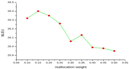
Figure 3: Experiment results on the test sets using different reallocation weights.
4.3 Effect of Reallocation Weightλ.
In Eq. (6), the reallocation weightλ determines which part plays a more important role in our method. In order to investigate the effect of λ
on our method, we tried different values for λ: from 0.1 to 0.5 with an increment of 0.05 each time. The experimental setup is the same as the previous experiments. Figure 3 shows the aver-age BLEU scores on the two test sets. Our sys-tem performs well whenλranges from0.1to0.25. The performance drops whenλis larger than0.25. A small reallocation weightλreduces the impact of initial evidences and local source-side associa-tions in the collective lexical selection algorithm, but increases the impact of global dependencies of target-side translation, which are normally not considered in previous lexical selection methods. This performance curve on the values of λ sug-gests that target-side global dependencies are im-portant for lexical selection.
5 Related Work
The collective inference algorithm is partially in-spired by Han et al. (2011) who propose a graph-based collective entity linking (EL) method to model global interdependences among different EL decisions. We successfully adapt this algo-rithm to lexical selection in SMT. Other related work mainly includes the following two strands.
(1) Lexical selection in SMT. In order to cap-ture source-side context for lexical selection, some researchers propose trigger-based lexicon models
to capture long-distance dependencies (Hasan et al., 2008; Mauser et al., 2009), and many more re-searchers build classifiers with rich context infor-mation to select desirable translations during de-coding (Chan et al., 2007; Carpuat and Wu, 2007; He et al., 2008; Liu et al., 2008). Shen et al. (2009) introduce four new linguistic and contextual
fea-tures for HPB system. We have also witnessed in-creasing efforts in the exploitation of document-level context information. Xiao et al. (2011) impose a hard constraint to guarantee the trans-lation consistency in document-level transtrans-lation. Ture et al. (2012) soften this consistency con-straint by integrating three counting features into decoder. Hardmeier et al. (2012, 2013) introduce a document-wide phrase-based decoder and inte-grate a semantic language model that cross sen-tence boundaries into the decoder. Based on topic models, Xiao et al. (2012) present a topic simi-larity model for HPB system, where each rule is assigned with a topic distribution. Also relevant is the work of Xiong et al. (2013), who use three different models to capture lexical cohesion for document-level machine translation. Compared with the above-mentioned studies, our method fo-cuses on the exploitation of global dependencies among target translations, which has attracted lit-tle attention before.
Different from exploring source-side context, other researchers pay attention to the utilization of target-side context information. The com-mon practice in SMT is to use an n-gram lan-guage model to capture local dependencies be-tween translations (Koehn et al., 2003; Xiong et al., 2011). Yet another approach exploring target-side context information is proposed by Shen et al. (2008), who use a dependency language model to capture long-distance relations on the target side. Moreover, Zhang et al. (2014) treat translation as an unconstrained target sentence generation task, using soft features to capture lexical and syntac-tic correspondences between the source and tar-get language. Recently, many researcher have proposed to use deep neural networks to model long-distance dependencies of arbitrary length for SMT (Auli et al., 2013; Kalchbrenner and Blun-som, 2013; Devlin et al., 2014; Hu et al., 2014; Liu et al., 2014; Sundermeyer et al., 2014). Our work is significantly different from these meth-ods. We use a graph representation to capture local and global context information, which, to the best of our knowledge, is the first attempt to explore graph-based representations for lexical selection. Furthermore, our model do not resort to any syn-tactic resources such as dependency parsers of the target language.
al-gorithm has been applied in SMT. For example, Cui et al. (2013) develop an effective approach to optimize phrase scoring and corpus weighting jointly using graph-based random walk. Zhu et al. (2013) apply a random walk method to dis-cover implicit relations between the phrases of dif-ferent languages. Aiming to better evaluate trans-lation quality at the document level, Gong and Li (2013) run PageRank algorithm to assign weights to words in translation evaluation. Different from these studies, the key interest of our research lies in the lexical selection with random walk.
6 Conclusion and Future Work
This paper has presented a novel graph-based collective lexical selection method for SMT. We build translation graphs to capture local source-side associations and global target-source-side dependen-cies, and propose a purely collective inference al-gorithm to jointly identify target translations of source-side content words in translation graphs. Our method capitalizes on capabilities of transla-tion graphs to represent both local and global rela-tions on the source/target side. Experiment results demonstrate the effectiveness of our method.
In the future, we plan to further improve our model by capturing semantic relatedness among source words. Additionally, we also want to jointly model different levels of context informa-tion in a unified framework for SMT.
Acknowledgments
The authors were supported by National Nat-ural Science Foundation of China (Grant Nos 61303082 and 61403269), Natural Science Foundation of Jiangsu Province (Grant No. BK20140355), Research Fund for the Doctoral Program of Higher Education of China (Grant No. 20120121120046), Research fund of the State Key Laboratory for Novel Software Technology in Nanjing University (Grant No. KFKT2015B11), the Special and Major Subject Project of the Industrial Science and Technology in Fujian Province 2013 (Grant No. 2013HZ0004-1), and 2014 Key Project of Anhui Science and Technology Bureau (Grant No. 1301021018). We also thank the anonymous reviewers for their insightful comments.
References
Michael Auli, Michel Galley, Chris Quirk, and Geof-frey Zweig. 2013. Joint language and translation modeling with recurrent neural networks. InProc. of EMNLP 2013, pages 1044–1054.
Marine Carpuat and Dekai Wu. 2007. Improving sta-tistical machine translation using word sense disam-biguation. InProc. of EMNLP 2007, pages 61–72. Yee Seng Chan, Hwee Tou Ng, and David Chiang.
2007. Word sense disambiguation improves statis-tical machine translation. In Proc. of ACL 2007, pages 33–40.
David Chiang. 2007. Hierarchical phrase-based trans-lation.Computational Linguistics, pages 201–228. Kenneth Ward Church and Patrick Hanks. 1990. Word
association norms, mutual information, and lexicog-raphy.Computational Linguistics, 16(1):22–29. Jonathan H. Clark, Chris Dyer, Alon Lavie, and
Noah A. Smith. 2011. Better hypothesis testing for statistical machine translation: Controlling for opti-mizer instability. In Proc. of ACL 2011, short pa-pers, pages 176–181.
Lei Cui, Dongdong Zhang, Shujie Liu, Mu Li, and Ming Zhou. 2013. Bilingual data cleaning for smt using graph-based random walk. In Proc. of ACL 2013, pages 340–345.
Jacob Devlin, Rabih Zbib, Zhongqiang Huang, Thomas Lamar, Richard Schwartz, and John Makhoul. 2014. Fast and robust neural network joint models for sta-tistical machine translation. InProc. of ACL 2014, pages 1370–1380.
F. Gobel and A.A. Jagers. 1974. Random walks on graphs. Stochastic Processes and Their Applica-tions, 2(4):331–336.
Zhengxian Gong and Liangyou Li. 2013. Document-level automatic machine translation evaluation based on weighted lexical cohesion. In Proc. of NLPCC 2013.
Xianpei Han, Le Sun, and Jun Zhao. 2011. Collective entity linking in web text: A graph-based method. InProc. of SIGIR 2011, pages 765–774.
Saˇsa Hasan, Juri Ganitkevitch, Hermann Ney, and Jes´us Andr´es-Ferrer. 2008. Triplet lexicon mod-els for statistical machine translation. In Proc. of EMNLP 2008, pages 372–381.
Zhongjun He, Qun Liu, and Shouxun Lin. 2008. Im-proving statistical machine translation using lexical-ized rule selection. InProc. of COLING 2008, pages 321–328.
Nal Kalchbrenner and Phil Blunsom. 2013. Recurrent continuous translation models. InProc. of EMNLP 2013, pages 1700–1709.
Philipp Koehn, Franz Josef Och, and Daniel Marcu. 2003. Statistical phrase-based translation. InProc. of NAACL-HLT 2003, pages 127–133.
Philipp Koehn. 2004. Statistical significance tests for machine translation evaluation. InProc. of EMNLP 2004, pages 388–395.
Qun Liu, Zhongjun He, Yang Liu, and Shouxun Lin. 2008. Maximum entropy based rule selection model for syntax-based statistical machine translation. In Proc. of EMNLP 2008, pages 89–97.
Kang Liu, Liheng Xu, and Jun Zhao. 2014. Extract-ing opinion targets and opinionwords from online re-views with graph co-ranking. InProc. of ACL 2014, pages 314–324.
Arne Mauser, Saˇsa Hasan, and Hermann Ney. 2009. Extending statistical machine translation with dis-criminative and trigger-based lexicon models. In Proc. of EMNLP 2009, pages 210–218.
Franz Joseph Och and Hermann Ney. 2003. A sys-tematic comparison of various statistical alignment models. Computational Linguistics, 29:19–51. Franz Joseph Och. 2003. Minimum error rate training
in statistical machine translation. In Proc. of ACL 2003, pages 160–167.
Kishore Papineni, Salim Roukos, Todd Ward, and Wei-Jing Zhu. 2002. Bleu: A method for automatic eval-uation of machine translation. InProc. of ACL 2002, pages 311–318.
Libin Shen, Jinxi Xu, and Ralph Weischedel. 2008. A new string-to-dependency machine translation algo-rithm with a target dependency language model. In Proc. of ACL 2008, pages 577–585.
Libin Shen, Jinxi Xu, Bing Zhang, Spyros Matsoukas, and Ralph Weischedel. 2009. Effective use of lin-guistic and contextual information for statistical ma-chine translation. InProc. of EMNLP 2009, pages 72–80.
Andreas Stolcke. 2002. Srilm - an extensible language modeling toolkit. In Proc. of ICSLP 2002, pages 901–904.
Martin Sundermeyer, Tamer Alkhouli, Joern Wuebker, and Hermann Ney. 2014. Translation modeling with bidirectional recurrent neural networks. In Proc. of EMNLP 2014, pages 14–25.
Ferhan Ture, DouglasW. Oard, and Philip Resnik. 2012. Encouraging consistent translation choices. InProc. of NAACL-HLT 2012, pages 417–426. Tong Xiao, Jingbo Zhu, Shujie Yao, and Hao Zhang.
2011. Document-level consistency verification in machine translation. InProc. of MT SUMMIT 2011, pages 131–138.
Xinyan Xiao, Deyi Xiong, Min Zhang, Qun Liu, and Shouxun Lin. 2012. A topic similarity model for hi-erarchical phrase-based translation. InProc. of ACL 2012, pages 750–758.
Deyi Xiong and Min Zhang. 2014. A sense-based translation model for statistical machine translation. InProc. of ACL 2014, pages 1459–1469.
Deyi Xiong, Min Zhang, and Haizhou Li. 2011. Enhancing language models in statistical machine translation with backward n-grams and mutual infor-mation triggers. InProc. of ACL 2011, pages 1288– 1297.
Deyi Xiong, Guosheng Ben, Min Zhang, Yajuan L¨u, and Qun Liu. 2013. Modeling lexical cohesion for document-level machine translation. InProc. of IJ-CAI 2013, pages 2183–2189.
Yue Zhang, Kai Song, Linfeng Song, Jingbo Zhu, and Qun Liu. 2014. Syntactic smt using a discriminative text generation model. In Proc. of EMNLP 2014, pages 177–182.