Effective Approaches to Attention based Neural Machine Translation

Effective Approaches to Attention-based Neural Machine Translation

Minh-Thang Luong Hieu Pham Christopher D. Manning Computer Science Department, Stanford University, Stanford, CA 94305

{lmthang,hyhieu,manning}@stanford.edu

Abstract

An attentional mechanism has lately been used to improve neural machine transla-tion (NMT) by selectively focusing on parts of the source sentence during trans-lation. However, there has been little work exploring useful architectures for attention-based NMT. This paper exam-ines two simple and effective classes of at-tentional mechanism: a global approach which always attends to all source words and alocalone that only looks at a subset of source words at a time. We demonstrate the effectiveness of both approaches on the WMT translation tasks between English and German in both directions. With local attention, we achieve a significant gain of 5.0 BLEU points over non-attentional sys-tems that already incorporate known tech-niques such as dropout. Our ensemble model using different attention architec-tures yields a new state-of-the-art result in the WMT’15 English to German transla-tion task with 25.9 BLEU points, an im-provement of 1.0 BLEU points over the existing best system backed by NMT and ann-gram reranker.1

1 Introduction

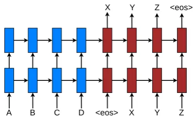
Neural Machine Translation (NMT) achieved state-of-the-art performances in large-scale trans-lation tasks such as from English to French (Luong et al., 2015) and English to German (Jean et al., 2015). NMT is appealing since it requires minimal domain knowledge and is conceptually simple. The model by Luong et al. (2015) reads through all the source words until the end-of-sentence symbol <eos>is reached. It then starts emitting one tar-get word at a time, as illustrated in Figure 1. NMT 1_{All our code and models are publicly available athttp:} //nlp.stanford.edu/projects/nmt.

B C D <eos> X Y Z

X Y Z <eos>

A

Figure 1: Neural machine translation – a stack-ing recurrent architecture for translatstack-ing a source sequence A B C D into a target sequence X Y Z. Here,<eos>marks the end of a sentence.

is often a large neural network that is trained in an end-to-end fashion and has the ability to general-ize well to very long word sequences. This means the model does not have to explicitly store gigantic phrase tables and language models as in the case of standard MT; hence, NMT has a small memory footprint. Lastly, implementing NMT decoders is easy unlike the highly intricate decoders in stan-dard MT (Koehn et al., 2003).

In parallel, the concept of “attention” has gained popularity recently in training neural networks, al-lowing models to learn alignments between dif-ferent modalities, e.g., between image objects and agent actions in the dynamic control problem (Mnih et al., 2014), between speech frames and text in the speech recognition task (Chorowski et al., 2014), or between visual features of a picture and its text description in the image caption gen-eration task (Xu et al., 2015). In the context of NMT, Bahdanau et al. (2015) has successfully ap-plied such attentional mechanism to jointly trans-late and align words. To the best of our knowl-edge, there has not been any other work exploring the use of attention-based architectures for NMT.

In this work, we design, with simplicity and ef-fectiveness in mind, two novel types of

based models: a global approach in which all source words are attended and alocalone whereby only a subset of source words are considered at a time. The former approach resembles the model of (Bahdanau et al., 2015) but is simpler architec-turally. The latter can be viewed as an interesting blend between thehardand softattention models proposed in (Xu et al., 2015): it is computation-ally less expensive than the global model or the soft attention; at the same time, unlike the hard at-tention, the local attention is differentiable, mak-ing it easier to implement and train.2 _{Besides, we} also examine various alignment functions for our attention-based models.

Experimentally, we demonstrate that both of our approaches are effective in the WMT trans-lation tasks between English and German in both directions. Our attentional models yield a boost of up to 5.0 BLEU over non-attentional systems which already incorporate known techniques such as dropout. For English to German translation, we achieve new state-of-the-art (SOTA) results for both WMT’14 and WMT’15, outperforming previous SOTA systems, backed by NMT mod-els and n-gram LM rerankers, by more than 1.0 BLEU. We conduct extensive analysis to evaluate our models in terms of learning, the ability to han-dle long sentences, choices of attentional architec-tures, alignment quality, and translation outputs.

2 Neural Machine Translation

A neural machine translation system is a neural network that directly models the conditional prob-ability p(y|x) of translating a source sentence, x1, . . . , xn, to a target sentence, y1, . . . , ym.3 A basic form of NMT consists of two components: (a) anencoderwhich computes a representations

for each source sentence and (b) adecoder which generates one target word at a time and hence de-composes the conditional probability as:

logp(y|x) =Xm_j=1logp(yj|y<j,s) (1)

A natural choice to model such a decomposi-tion in the decoder is to use a recurrent neural net-work (RNN) architecture, which most of the re-2_{There is a recent work by Gregor et al. (2015), which is} very similar to our local attention and applied to the image generation task. However, as we detail later, our model is much simpler and can achieve good performance for NMT.

3_{All sentences are assumed to terminate with a special} “end-of-sentence” token<eos>.

cent NMT work such as (Kalchbrenner and Blun-som, 2013; Sutskever et al., 2014; Cho et al., 2014; Bahdanau et al., 2015; Luong et al., 2015; Jean et al., 2015) have in common. They, however, dif-fer in terms of which RNN architectures are used for the decoder and how the encoder computes the source sentence representations.

Kalchbrenner and Blunsom (2013) used an RNN with the standard hidden unit for the decoder and a convolutional neural network for encoding the source sentence representation. On the other hand, both Sutskever et al. (2014) and Luong et al. (2015) stacked multiple layers of an RNN with a Long Short-Term Memory (LSTM) hidden unit for both the encoder and the decoder. Cho et al. (2014), Bahdanau et al. (2015), and Jean et al. (2015) all adopted a different version of the RNN with an LSTM-inspired hidden unit, the gated re-current unit (GRU), for both components.4

In more detail, one can parameterize the proba-bility of decoding each wordyj as:

p(yj|y<j,s) = softmax (g(hj)) (2) withgbeing the transformation function that out-puts a vocabulary-sized vector.5 _{Here, h}

j is the RNN hidden unit, abstractly computed as:

hj =f(hj−1,s), (3) where f computes the current hidden state given the previous hidden state and can be either a vanilla RNN unit, a GRU, or an LSTM unit. In (Kalchbrenner and Blunsom, 2013; Sutskever et al., 2014; Cho et al., 2014; Luong et al., 2015), the source representation s is only used once to initialize the decoder hidden state. On the other hand, in (Bahdanau et al., 2015; Jean et al., 2015) and this work, s, in fact, implies a set of source hidden states which are consulted throughout the entire course of the translation process. Such an approach is referred to as an attention mechanism, which we will discuss next.

In this work, following (Sutskever et al., 2014; Luong et al., 2015), we use the stacking LSTM architecture for our NMT systems, as illustrated in Figure 1. We use the LSTM unit defined in (Zaremba et al., 2015). Our training objective is formulated as follows:

Jt=

X

(x,y)∈D−logp(y|x) (4) 4_{They all used a single RNN layer except for the latter two} works which utilized a bidirectional RNN for the encoder.

withDbeing our parallel training corpus. 3 Attention-based Models

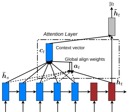
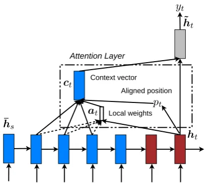
Our various attention-based models are classifed into two broad categories,globalandlocal. These classes differ in terms of whether the “attention” is placed on all source positions or on only a few source positions. We illustrate these two model types in Figure 2 and 3 respectively.

Common to these two types of models is the fact that at each time steptin the decoding phase, both approaches first take as input the hidden stateht at the top layer of a stacking LSTM. The goal is then to derive a context vectorctthat captures rel-evant source-side information to help predict the current target wordyt. While these models differ in how the context vectorctis derived, they share the same subsequent steps.

Specifically, given the target hidden statehtand the source-side context vector ct, we employ a simple concatenation layer to combine the infor-mation from both vectors to produce an attentional hidden state as follows:

˜

ht= tanh(Wc[ct;ht]) (5)

The attentional vector˜htis then fed through the softmax layer to produce the predictive distribu-tion formulated as:

p(yt|y<t, x) = softmax(Wsh˜t) (6)

We now detail how each model type computes the source-side context vectorct.

3.1 Global Attention

The idea of a global attentional model is to con-sider all the hidden states of the encoder when de-riving the context vector ct. In this model type, a variable-length alignment vectorat, whose size equals the number of time steps on the source side, is derived by comparing the current target hidden statehtwith each source hidden stateh¯s:

at(s) = align(ht,¯hs) (7)

= exp score(ht,h¯s) P

s′exp score(h_t,¯h_s′)

Here,scoreis referred as acontent-basedfunction for which we consider three different alternatives:

score(ht,¯hs) =

    

h⊤

t ¯hs dot

h⊤_t Wah¯s general

Wa[ht;¯hs] concat

(8)

yt

˜

ht

ct

at

ht

¯

hs

Global align weights

Attention Layer

Context vector

Figure 2:Global attentional model– at each time step t, the model infers a variable-length align-ment weight vectoratbased on the current target statehtand all source states¯hs. A global context vector ctis then computed as the weighted aver-age, according toat, over all the source states.

Besides, in our early attempts to build attention-based models, we use a location-based function in which the alignment scores are computed from solely the target hidden statehtas follows:

at= softmax(Waht) location (9)

Given the alignment vector as weights, the context vectorctis computed as the weighted average over all the source hidden states.6

Comparison to (Bahdanau et al., 2015)– While

our global attention approach is similar in spirit to the model proposed by Bahdanau et al. (2015), there are several key differences which reflect how we have both simplified and generalized from the original model. First, we simply use hidden states at the top LSTM layers in both the encoder and decoder as illustrated in Figure 2. Bahdanau et al. (2015), on the other hand, use the concatena-tion of the forward and backward source hidden states in the bi-directional encoder and target hid-den states in their non-stacking uni-directional de-coder. Second, our computation path is simpler; we go from ht → at → ct → ˜ht then make a prediction as detailed in Eq. (5), Eq. (6), and Figure 2. On the other hand, at any timet, Bah-danau et al. (2015) build from the previous hidden state ht−1 → at → ct → ht, which, in turn,

6_{Eq. (9) implies that all alignment vectorsa}

tare of the

yt

˜

ht

ct

at

ht

pt

¯

hs

Attention Layer

Context vector

Local weights Aligned position

Figure 3: Local attention model– the model first predicts a single aligned positionptfor the current target word. A window centered around the source positionptis then used to compute a context vec-tor ct, a weighted average of the source hidden states in the window. The weightsatare inferred

from the current target state htand those source states¯hsin the window.

goes through a deep-output and a maxout layer before making predictions.7 _{Lastly, Bahdanau et} al. (2015) only experimented with one alignment function, the concat product; whereas we show later that the other alternatives are better.

3.2 Local Attention

The global attention has a drawback that it has to attend to all words on the source side for each tar-get word, which is expensive and can potentially render it impractical to translate longer sequences, e.g., paragraphs or documents. To address this deficiency, we propose a local attentional mech-anism that chooses to focus only on a small subset of the source positions per target word.

This model takes inspiration from the tradeoff between thesoftandhardattentional models pro-posed by Xu et al. (2015) to tackle the image cap-tion generacap-tion task. In their work, soft attencap-tion refers to the global attention approach in which weights are placed “softly” over all patches in the source image. The hard attention, on the other hand, selects one patch of the image to attend to at a time. While less expensive at inference time, the hard attention model is non-differentiable and re-quires more complicated techniques such as vari-ance reduction or reinforcement learning to train.

7_{We will refer to this difference again in Section 3.3.}

Our local attention mechanism selectively fo-cuses on a small window of context and is differ-entiable. This approach has an advantage of avoid-ing the expensive computation incurred in the soft attention and at the same time, is easier to train than the hard attention approach. In concrete de-tails, the model first generates an aligned position ptfor each target word at timet. The context vec-tor ct is then derived as a weighted average over the set of source hidden states within the window

[pt−D, pt+D];Dis empirically selected.8 Unlike the global approach, the local alignment vectorat is now fixed-dimensional, i.e.,∈R2D+1_{. We} con-sider two variants of the model as below.

Monotonicalignment (local-m) – we simply set pt=tassuming that source and target sequences are roughly monotonically aligned. The alignment vectoratis defined according to Eq. (7).9

Predictive alignment (local-p) – instead of as-suming monotonic alignments, our model predicts an aligned position as follows:

pt=S·sigmoid(vp⊤tanh(Wpht)), (10)

Wp and vp are the model parameters which will

be learned to predict positions. Sis the source sen-tence length. As a result ofsigmoid,pt ∈ [0, S]. To favor alignment points near pt, we place a Gaussian distribution centered aroundpt. Specif-ically, our alignment weights are now defined as:

at(s) = align(ht,h¯s) exp

−(s−pt)2

2σ2

(11)

We use the samealign function as in Eq. (7) and the standard deviation is empirically set asσ=D

2. It is important to note that pt is arealnummber; whereas s is an integer within the window cen-tered atpt.10

Comparison to (Gregor et al., 2015)– have pro-posed aselective attention mechanism, very simi-lar to our local attention, for the image generation task. Their approach allows the model to select an image patch of varying location and zoom. We, instead, use the same “zoom” for all target posi-tions, which greatly simplifies the formulation and still achieves good performance.

8_{If the window crosses the sentence boundaries, we} sim-ply ignore the outside part and consider words in the window. 9_{local-mis the same as the global model except that the} vectora_tis fixed-length and shorter.

10_{local-p is similar to the local-m model except that we} dynamically compute pt and use a Gaussian distribution

˜

ht

Attention Layer

B C D <eos> X Y Z

X Y Z <eos>

A

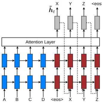
Figure 4: Input-feeding approach – Attentional vectorsh˜tare fed as inputs to the next time steps to inform the model about past alignment decisions.

3.3 Input-feeding Approach

In our proposed global and local approaches, the attentional decisions are made independently, which is suboptimal. Whereas, in standard MT,

a coverage set is often maintained during the

translation process to keep track of which source words have been translated. Likewise, in atten-tional NMTs, alignment decisions should be made jointly taking into account past alignment infor-mation. To address that, we propose an input-feeding approach in which attentional vectors h˜t are concatenated with inputs at the next time steps as illustrated in Figure 4.11 _{The effects of} hav-ing such connections are two-fold: (a) we hope to make the model fully aware of previous align-ment choices and (b) we create a very deep net-work spanning both horizontally and vertically.

Comparison to other work – Bahdanau et al.

(2015) use context vectors, similar to our ct, in building subsequent hidden states, which can also achieve the “coverage” effect. However, there has not been any analysis of whether such connections are useful as done in this work. Also, our approach is more general; as illustrated in Figure 4, it can be applied to general stacking recurrent architectures, including non-attentional models.

Xu et al. (2015) propose a doubly attentional

approach with an additional constraint added to the training objective to make sure the model pays equal attention to all parts of the image during the caption generation process. Such a constraint can 11_{Ifnis the number of LSTM cells, the input size of the} first LSTM layer is2n; those of subsequent layers aren.

also be useful to capture the coverage set effect in NMT that we mentioned earlier. However, we chose to use the input-feeding approach since it provides flexibility for the model to decide on any attentional constraints it deems suitable.

4 Experiments

We evaluate the effectiveness of our models on the WMT translation tasks between English and Ger-man in both directions. newstest2013 (3000 sen-tences) is used as a development set to select our hyperparameters. Translation performances are reported in case-sensitive BLEU (Papineni et al., 2002) on newstest2014 (2737 sentences) and new-stest2015 (2169 sentences). Following (Luong et al., 2015), we report translation quality using two types of BLEU: (a)tokenized12 _{BLEU to be} com-parable with existing NMT work and (b) NIST13 BLEU to be comparable with WMT results.

4.1 Training Details

All our models are trained on the WMT’14 train-ing data consisttrain-ing of 4.5M sentences pairs (116M English words, 110M German words). Similar to (Jean et al., 2015), we limit our vocabularies to be the top 50K most frequent words for both lan-guages. Words not in these shortlisted vocabular-ies are converted into a universal token<unk>.

When training our NMT systems, following (Bahdanau et al., 2015; Jean et al., 2015), we fil-ter out sentence pairs whose lengths exceed 50 words and shuffle mini-batches as we proceed. Our stacking LSTM models have 4 layers, each with 1000 cells, and 1000-dimensional embed-dings. We follow (Sutskever et al., 2014; Luong et al., 2015) in training NMT with similar set-tings: (a) our parameters are uniformly initialized in [−0.1,0.1], (b) we train for 10 epochs using plain SGD, (c) a simple learning rate schedule is employed – we start with a learning rate of 1; after 5 epochs, we begin to halve the learning rate ev-ery epoch, (d) our mini-batch size is 128, and (e) the normalized gradient is rescaled whenever its norm exceeds 5. Additionally, we also use dropout for our LSTMs as suggested by (Zaremba et al., 2015). For dropout models, we train for 12 epochs and start halving the learning rate after 8 epochs.

Our code is implemented in MATLAB. When 12_{All texts are tokenized with tokenizer.perl and} BLEU scores are computed withmulti-bleu.perl.

System Ppl BLEU

Winning WMT’14 system –phrase-based + large LM(Buck et al., 2014) 20.7

Existing NMT systems

RNNsearch (Jean et al., 2015) 16.5

RNNsearch + unk replace (Jean et al., 2015) 19.0

RNNsearch + unk replace + large vocab +ensemble8 models (Jean et al., 2015) 21.6

Our NMT systems

Base 10.6 11.3

Base + reverse 9.9 12.6 (+1.3)

Base + reverse + dropout 8.1 14.0 (+1.4)

Base + reverse + dropout + global attention (location) 7.3 16.8 (+2.8)

Base + reverse + dropout + global attention (location) + feed input 6.4 18.1 (+1.3)

Base + reverse + dropout + local-p attention (general) + feed input _{5.9 19.0 (}+0.9)

Base + reverse + dropout + local-p attention (general) + feed input + unk replace 20.9 (+1.9)

Ensemble8 models + unk replace 23.0 (+2.1)

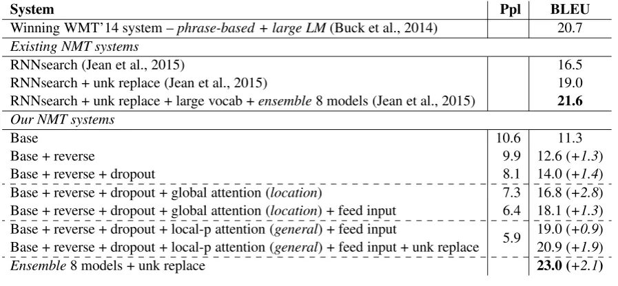
Table 1:WMT’14 English-German results– shown are the perplexities (ppl) and thetokenizedBLEU scores of various systems on newstest2014. We highlight thebestsystem in bold and giveprogressive

improvements in italic between consecutive systems. local-preferes to the local attention with predictive alignments. We indicate for each attention model the alignment score function used in pararentheses.

running on a single GPU device Tesla K40, we achieve a speed of 1K target words per second. It takes 7–10 days to completely train a model. 4.2 English-German Results

We compare our NMT systems in the English-German task with various other systems. These include the winning system in WMT’14 (Buck et al., 2014), a phrase-based system whose language models were trained on a huge monolingual text, the Common Crawl corpus. For end-to-end neu-ral machine translation systems, to the best of our knowledge, (Jean et al., 2015) is the only work ex-perimenting with this language pair and currently the SOTA system. We only present results for some of our attention models and will later ana-lyze the rest in Section 5.

As shown in Table 1, we achieve progressive improvements when (a) reversing the source sen-tence, +1.3 BLEU, as proposed in (Sutskever et al., 2014) and (b) using dropout, +1.4BLEU. On top of that, (c) the global attention approach gives a significant boost of +2.8 BLEU, making our model slightly better than the base attentional sys-tem of Bahdanau et al. (2015) (row RNNSearch). When (d) using the input-feeding approach, we seize another notable gain of +1.3BLEU and out-perform their system. The local attention model with predictive alignments (row local-p) proves to be even better, giving us a further improve-ment of +0.9BLEU on top of the global attention

model. It is interesting to observe the trend pre-viously reported in (Luong et al., 2015) that per-plexity strongly correlates with translation quality. In total, we achieve a significant gain of 5.0 BLEU points over the non-attentional baseline, which al-ready includes known techniques such as source reversing and dropout.

The unknown replacement technique proposed in (Luong et al., 2015; Jean et al., 2015) yields another nice gain of +1.9 BLEU, demonstrating that our attentional models do learn useful align-ments for unknown works. Finally, by ensembling 8 different models of various settings, e.g., using different attention approaches, with and without dropout etc., we were able to achieve anew SOTA

result of 23.0 BLEU, outperforming the existing best system (Jean et al., 2015) by +1.4BLEU.

System BLEU

SOTA –NMT + 5-gram rerank(MILA) 24.9

Our ensemble 8 models + unk replace 25.9

Table 2: WMT’15 English-German results –

NISTBLEU scores of the existing WMT’15 SOTA system and our best one on newstest2015.

es-System Ppl. BLEU

WMT’15 systems

SOTA –phrase-based(Edinburgh) 29.2 NMT + 5-gram rerank (MILA) 27.6

Our NMT systems

Base (reverse) 14.3 16.9

+ global (location) 12.7 19.1 (+2.2) + global (location) + feed 10.9 20.1 (+1.0) + global (dot) + drop + feed _{9.7 22.8 (}+2.7) + global (dot) + drop + feed + unk 24.9 (+2.1)

Table 3: WMT’15 German-English results – performances of various systems (similar to Ta-ble 1). The base system already includes source reversing on which we add global attention,

dropout, inputfeeding, andunkreplacement.

tablishes anew SOTAperformance of25.9BLEU, outperforming the existing best system backed by NMT and a 5-gram LM reranker by +1.0BLEU.

4.3 German-English Results

We carry out a similar set of experiments for the WMT’15 translation task from German to En-glish. While our systems have not yet matched the performance of the SOTA system, we never-theless show the effectiveness of our approaches with large and progressive gains in terms of BLEU as illustrated in Table 3. The attentional mech-anism gives us +2.2 BLEU gain and on top of that, we obtain another boost of up to +1.0BLEU from the input-feeding approach. Using a better alignment function, the content-baseddotproduct one, together withdropoutyields another gain of +2.7 BLEU. Lastly, when applying the unknown word replacement technique, we seize an addi-tional +2.1 BLEU, demonstrating the usefulness of attention in aligning rare words.

5 Analysis

We conduct extensive analysis to better understand our models in terms of learning, the ability to han-dle long sentences, choices of attentional archi-tectures, and alignment quality. All models con-sidered here are English-German NMT systems tested on newstest2014.

5.1 Learning curves

We compare models built on top of one another as listed in Table 1. It is pleasant to observe in Fig-ure 5 a clear separation between non-attentional and attentional models. The input-feeding

ap-0.2 0.4 0.6 0.8 1 1.2 1.4 1.6 1.8 x 105 2

3 4 5 6

Mini−batches

Test cost

basic basic+reverse basic+reverse+dropout basic+reverse+dropout+globalAttn basic+reverse+dropout+globalAttn+feedInput basic+reverse+dropout+pLocalAttn+feedInput

Figure 5:Learning curves– test cost (ln perplex-ity) on newstest2014 for English-German NMTs as training progresses.

proach and the local attention model also demon-strate their abilities in driving the test costs lower. The non-attentional model with dropout (the blue + curve) learns slower than other non-dropout models, but as time goes by, it becomes more ro-bust in terms of minimizing test errors.

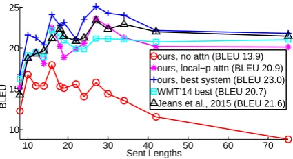
5.2 Effects of Translating Long Sentences We follow (Bahdanau et al., 2015) to group sen-tences of similar lengths together and compute a BLEU score per group. As demonstrated in Fig-ure 6, our attentional models are more effective than the other non-attentional model in handling long sentences: the translation quality does not de-grade as sentences become longer. Our best model (the blue + curve) outperforms all other systems in all length buckets.

10 20 30 40 50 60 70

10 15 20 25

Sent Lengths

BLEU

ours, no attn (BLEU 13.9) ours, local−p attn (BLEU 20.9) ours, best system (BLEU 23.0) WMT’14 best (BLEU 20.7) Jeans et al., 2015 (BLEU 21.6)

Figure 6: Length Analysis– translation qualities of different systems as sentences become longer.

5.3 Choices of Attentional Architectures We examine different attention models (global,

local-m, local-p) and different alignment

System Ppl _BeforeBLEU_{After unk} global (location) 6.4 18.1 19.3 (+1.2) global (dot) 6.1 18.6 20.5 (+1.9) global (general) 6.1 17.3 19.1 (+1.8) local-m (dot) >7.0 x x local-m (general) 6.2 18.6 20.4 (+1.8) local-p (dot) 6.6 18.0 19.6 (+1.9) local-p (general) 5.9 19 20.9 (+1.9)

Table 4: Attentional Architectures – perfor-mances of different attentional models. We trained two local-m (dot) models; both have ppl>7.0.

results in Table 4 do give us some idea about dif-ferent choices. The location-based function does not learn good alignments: the global (location)

model can only obtain a small gain when perform-ing unknown word replacement compared to usperform-ing other alignment functions.14 _{For content-based} functions, our implementation ofconcat does not yield good performances and more analysis should be done to understand the reason.15 _{It is} interest-ing to observe that dot works well for the global attention andgeneral is better for the local tion. Among the different models, the local atten-tion model with predictive alignments (local-p) is best, both in terms of perplexities and BLEU.

5.4 Alignment Quality

A by-product of attentional models are word align-ments. While (Bahdanau et al., 2015) visualized alignments for some sample sentences and ob-served gains in translation quality as an indica-tion of a working attenindica-tion model, no work has as-sessed the alignments learned as a whole. In con-trast, we set out to evaluate the alignment quality using the alignment error rate (AER) metric.

Given the gold alignment data provided by RWTH for 508 English-German Europarl sen-tences, we “force” decode our attentional models to produce translations that match the references. We extract only one-to-one alignments by select-ing the source word with the highest alignment 14_{There is a subtle difference in how we retrieve} align-ments for the different alignment functions. At time steptin which we receiveyt−1as input and then computeh_t,a_t,c_t, andh˜_tbefore predictingy_t, the alignment vectora_tis used as alignment weights for (a) the predicted wordyt in the location-basedalignment functions and (b) the input word yt−1in thecontent-basedfunctions.

15_{Withconcat, the perplexities achieved by different} mod-els are 6.7 (global), 7.1 (local-m), and 7.1 (local-p).

Method AER

global (location) 0.39

local-m (general) 0.34

local-p (general) 0.36

ensemble 0.34

Berkeley Aligner 0.32

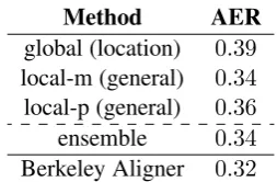
Table 6: AER scores– results of various models on the RWTH English-German alignment data.

weight per target word. Nevertheless, as shown in Table 6, we were able to achieve AER scores com-parable to the one-to-many alignments obtained by the Berkeley aligner (Liang et al., 2006).16

We also found that the alignments produced by local attention models achieve lower AERs than those of the global one. The AER obtained by the ensemble, while good, is not better than the local-m AER, suggesting the well-known observa-tion that AER and translaobserva-tion scores are not well correlated (Fraser and Marcu, 2007). Due to space constraint, we can only show alignment visualiza-tions in the arXiv version of our paper.17

5.5 Sample Translations

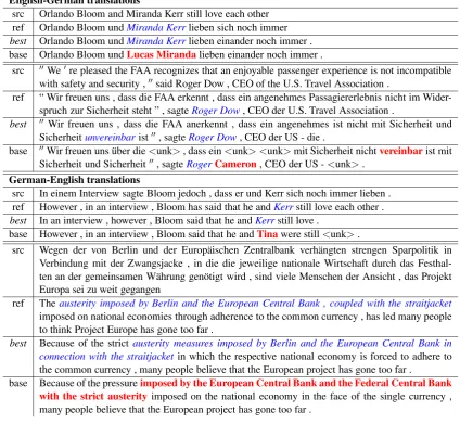
We show in Table 5 sample translations in both directions. It it appealing to observe the ef-fect of attentional models in correctly translat-ing names such as “Miranda Kerr” and “Roger Dow”. Non-attentional models, while producing sensible names from a language model perspec-tive, lack the direct connections from the source side to make correct translations.

We also observed an interesting case in the second English-German example, which requires translating the doubly-negated phrase, “not in-compatible”. The attentional model correctly produces “nicht . . . unvereinbar”; whereas the non-attentional model generates “nicht vereinbar”, meaning “not compatible”.18 _{The attentional} model also demonstrates its superiority in trans-lating long sentences as in the last example. 6 Conclusion

In this paper, we propose two simple and effec-tive attentional mechanisms for neural machine 16_{We concatenate the 508 sentence pairs with 1M sentence} pairs from WMT and run the Berkeley aligner.

17_{http://arxiv.org/abs/1508.04025}

English-German translations

src Orlando Bloom and Miranda Kerr still love each other ref Orlando Bloom undMiranda Kerrlieben sich noch immer

best Orlando Bloom undMiranda Kerrlieben einander noch immer . base Orlando Bloom undLucas Mirandalieben einander noch immer .

src ′′_We′_{re pleased the FAA recognizes that an enjoyable passenger experience is not incompatible}

with safety and security ,′′_{said Roger Dow , CEO of the U.S. Travel Association .}

ref “ Wir freuen uns , dass die FAA erkennt , dass ein angenehmes Passagiererlebnis nicht im Wider-spruch zur Sicherheit steht ” , sagteRoger Dow, CEO der U.S. Travel Association .

best ′′ _{Wir freuen uns , dass die FAA anerkennt , dass ein angenehmes ist nicht mit Sicherheit und}

Sicherheitunvereinbarist′′_{, sagteRoger Dow, CEO der US - die .}

base ′′_{Wir freuen uns ¨uber die<unk>, dass ein<unk> <unk>mit Sicherheit nichtvereinbarist mit}

Sicherheit und Sicherheit′′_{, sagteRogerCameron, CEO der US -<unk>.}

German-English translations

src In einem Interview sagte Bloom jedoch , dass er und Kerr sich noch immer lieben . ref However , in an interview , Bloom has said that he andKerrstill love each other .

best In an interview , however , Bloom said that he andKerrstill love .

base However , in an interview , Bloom said that he andTinawere still<unk>.

src Wegen der von Berlin und der Europ¨aischen Zentralbank verh¨angten strengen Sparpolitik in Verbindung mit der Zwangsjacke , in die die jeweilige nationale Wirtschaft durch das Festhal-ten an der gemeinsamen W¨ahrung gen¨otigt wird , sind viele Menschen der Ansicht , das Projekt Europa sei zu weit gegangen

ref Theausterity imposed by Berlin and the European Central Bank , coupled with the straitjacket

imposed on national economies through adherence to the common currency , has led many people to think Project Europe has gone too far .

best Because of the strict austerity measures imposed by Berlin and the European Central Bank in connection with the straitjacket in which the respective national economy is forced to adhere to the common currency , many people believe that the European project has gone too far .

base Because of the pressureimposed by the European Central Bank and the Federal Central Bank with the strict austerity imposed on the national economy in the face of the single currency , many people believe that the European project has gone too far .

Table 5:Sample translations– for each example, we show the source (src), the human translation (ref), the translation from our best model (best), and the translation of a non-attentional model (base). We italicize somecorrecttranslation segments and highlight a fewwrongones in bold.

translation: the global approach which always looks at all source positions and the local one that only attends to a subset of source positions at a time. We test the effectiveness of our mod-els in the WMT translation tasks between En-glish and German in both directions. Our local attention yields large gains of up to 5.0 BLEU over non-attentional models that already incorpo-rate known techniques such as dropout. For the English to German translation direction, our en-semble model has established new state-of-the-art results for both WMT’14 and WMT’15.

We have compared various alignment functions and shed light on which functions are best for which attentional models. Our analysis shows that attention-based NMT models are superior to non-attentional ones in many cases, for example in

translating names and handling long sentences.

Acknowledgment

References

Dzmitry Bahdanau, Kyunghyun Cho, and Yoshua Ben-gio. 2015. Neural machine translation by jointly learning to align and translate. InICLR.

Christian Buck, Kenneth Heafield, and Bas van Ooyen. 2014. N-gram counts and language models from the common crawl. InLREC.

Kyunghyun Cho, Bart van Merrienboer, Caglar Gul-cehre, Fethi Bougares, Holger Schwenk, and Yoshua Bengio. 2014. Learning phrase representations using RNN encoder-decoder for statistical machine translation. InEMNLP.

Jan Chorowski, Dzmitry Bahdanau, Kyunghyun Cho, and Yoshua Bengio. 2014. End-to-end continuous speech recognition using attention-based recurrent NN: first results.CoRR, abs/1412.1602.

Alexander Fraser and Daniel Marcu. 2007. Measuring word alignment quality for statistical machine trans-lation.Computational Linguistics, 33(3):293–303. Karol Gregor, Ivo Danihelka, Alex Graves,

Danilo Jimenez Rezende, and Daan Wierstra. 2015. DRAW: A recurrent neural network for image generation. InICML.

S´ebastien Jean, Kyunghyun Cho, Roland Memisevic, and Yoshua Bengio. 2015. On using very large tar-get vocabulary for neural machine translation. In

ACL.

Nal Kalchbrenner and Phil Blunsom. 2013. Recurrent continuous translation models. InEMNLP.

Philipp Koehn, Franz Josef Och, and Daniel Marcu. 2003. Statistical phrase-based translation. In

NAACL.

Percy Liang, Ben Taskar, and Dan Klein. 2006. Align-ment by agreeAlign-ment. InNAACL.

Minh-Thang Luong, Ilya Sutskever, Quoc V. Le, Oriol Vinyals, and Wojciech Zaremba. 2015. Addressing the rare word problem in neural machine translation. InACL.

Volodymyr Mnih, Nicolas Heess, Alex Graves, and Ko-ray Kavukcuoglu. 2014. Recurrent models of visual attention. InNIPS.

Kishore Papineni, Salim Roukos, Todd Ward, and Wei jing Zhu. 2002. Bleu: a method for automatic eval-uation of machine translation. InACL.

Ilya Sutskever, Oriol Vinyals, and Quoc V. Le. 2014. Sequence to sequence learning with neural net-works. InNIPS.

Kelvin Xu, Jimmy Ba, Ryan Kiros, Kyunghyun Cho, Aaron C. Courville, Ruslan Salakhutdinov, Richard S. Zemel, and Yoshua Bengio. 2015. Show, attend and tell: Neural image caption generation with visual attention. InICML.

Wojciech Zaremba, Ilya Sutskever, and Oriol Vinyals. 2015. Recurrent neural network regularization. In