Abstract— From a machine output torque point of view, the behaviour of a six-pole, nine slots, and chorded stator winding permanent magnet brushless dc (PMBLDC) machine is analysed in this article. To that end, the magnetostatic analysis capability of the two dimensional commercially available finite element modelling Package QuickField is employed. The simulation results on a 60 W Brushless dc motor show that the electromagnetic torque is effectively computed albeit further investigations to obtain a more accurate cogging torque may be considered.
Index Terms— PMBLDC, Torque, Magnetostatic analysis
I. INTRODUCTION
HE literature on permanent magnet brushless direct current (PMBLDC) machines is now so extensive as to witness the growing attention put on this type of rotating machinery. Some times encountered as motors of several thousand horsepower [1], they are also used as a small horsepower control motors for a wide variety of applications [2]. Among the main factors that have contributed to the above mentioned attraction there is the achievement of maximum power density [1]. Additionally, the elimination of brushes and slip rings brought by the replacement of electrical excitation with permanent magnets has made available economical designs with simpler construction, lower weight and size for the same performance. They also exhibit trapezoidal flux density distribution and phase voltages [3]; the BLDC motor retains the characteristics of a dc motor but eliminates the commutator and the brushes [4]. However, due to imperfections in commutation, there is considerable torque ripple that is the source of vibration and
Manuscript received February 08, 2013; revised February 21, 2013. G. M’boungui. is with the Department of Electrical Engineering Tshwane University of Technology
Private Bag X680, Pretoria 0001,Republic of South Africa phone: 078-497-2424; e-mail: [email protected]. E. K. Appiah is with the Department of Electrical Engineering Tshwane University of Technology
Private Bag X680, Pretoria 0001,Republic of South Africa e-mail: [email protected]
A. A. Jimoh is with the Department of Electrical Engineering Tshwane University of Technology
Private Bag X680, Pretoria 0001,Republic of South Africa e-mail: [email protected]
T. R. Ayodele is with the Department of Electrical Engineering Tshwane University of Technology
Private Bag X680, Pretoria 0001,Republic of South Africa e-mail: [email protected]
noise setting a limitation on their performance in applications where high precision in position and speed control is required [3] In addressing the issue of torque ripple reduction in PM BLDC some researchers have considered the problem mainly from electro-mechanical and electro-magnetic design aspects [5] while others have approached the problem from the drive and control perspective with the use of 2 or 3 Dimensional (2 or 3D) Finite Element Analysis (FEA). Field solvers are resorted to extensively in determination and evaluation of PMBLDC electric machines performance characteristics. Of utmost importance, the torque calculation is so often presented in formats that appear unintelligible to the uninitiated as in [6] for example. Therein lies a problem.
Among various arrangements of permanent magnets in BLDC motors, the popular surface mount arrangement with modern high coercive force magnet materials is chosen for the study. In this paper we specifically present the results of a short investigation, using the magnetostatic analysis capability of QuickField, a PC-oriented interactive environment for electromagnetic, thermal and stress analysis [7], on a 60 W, six-pole, 3-phase BLDC motor with a more friendly presentation of motor output torque computation.
The magnetostatic problem formulation will first be briefly reviewed. This is a mathematical property description of a domain, i.e. the motor comprising stator iron, stator windings, rotor yoke, permanent magnets and air, all subject to static or slowly varying in time (quasi-static) magnetic fields. Then, the geometry of the PMBLDC motor is presented and the magnetic field is theoretically analysed. Also, due to the influence of the armature currents on the output torque and its calculation, the motor power supply is described before the simulation of the motor which the results are presented and discussed.
II. MAGNETIC PROBLEM FORMULATION
Magnetic fields may be induced by the concentrated or distributed currents, permanent magnets or external magnetic fields.
It is assumed that flux density components lie in the plane of the model (xy), whereas the vector of electric current density J and the vector potential A are orthogonal to the flux density. Only the z components of J and A in planar case are non zero. The equation for planar case is [7]:
y H x H J y A y x A x
cx cy x
y
1
1 (1)
Simple Numerical Two Dimensional
Magnetostatic Analysis of a Fractional Slot
Winding Brushless DC Motor
G. M’boungui, E. K. Appiah, A. A. Jimoh, T. R. Ayodele
Where
x and
y,H
cxandH
cy are respectively components of magnitude permeability tensor and components of coercive force vector.Indeed according to Maxwell equations, a magnetic potential vector A may be defined as [8]:
A
B
(2) So that computing and finding A, B (magnetic field) can easily be determined from this definition. Also, the quasi-static form of Ampere’s law that is very important in the design of electric machine can be expressed as:J
H
(3) The term “quasi-static” indicates that the frequency of the phenomenon in question is low enough to neglect Maxwell current displacement. The phenomenon occurring in electrical machines meet the quasi-static requirement well [8].By applying permeability μ, we can describe materials by:
H
B
(4)Bringing (4) into (3) and combining with (2) the equations above yields
J
A
X
1
(5)Which, if μ is constant can be written under the form of three separate instances of the Poisson’s equation. Therefore, in 2D planar coordinates where the z components of J and A are non-zero, equation (5) becomes a single Poisson equation: z z z z J y A y x A x
A
1 1 1
. (6)
Next, the contribution Jb of Hc related to the current
density from the permanent magnet material may be expressed as k y H x H j x H z H i z H y H H
J cz cy cx cz cy cx
c b (7) With the k component only non-zero in the above equation, equation (1) may be re written
z z z
z y J
A y x A x
A
1 1 1 .
y
H
x
H
cy cx(8) Giving
j
x
A
i
y
A
A
B
z z
(9)III. MOTOR GEOMETRY DESCRIPTION AND ANALYSIS OF THE MAGNETIC FIELD
The Finite Element Analysis using 2D solver has been broadly used to determine and evaluate the performance of electrical machines performance characteristics [5]. In this article the aim is to explore only magnetostatic capability of QiuckField to solve linear and non-linear problem without the use of particular resources such as mesh refinement for example.
A. Motor description
[image:2.595.314.543.50.163.2]The six-pole BLDC machine under study having Ferrite Permanent magnets on the rotor has the cross section shown in figure 1. The motor data are reported in table 1.
Table 1: Motor data Stator data
Stator external diameter [mm] 125
Stator inner diameter [mm] 61
Stack length l [mm] 38
Number of poles [ ] 6
Number of slots [ ] 9
Number of series conductors per phase
[ ] 1456
Stator slots data
Width of slot opening b1 [mm] 3.55
Total height of slot [mm] 7.5
Rotor data 4
Rotor external diameter [mm] 22
Shaft diameter [mm] 44.7
Permanent magnet data
Permanent magnet thickness lm [mm] 7.5
Mechanical permanent magnet angle
[deg.] 55
Residual flux density (Ferrite) Br [T] 0.4
The stator structure is similar to that of a typical 3-phase, wye connected induction motor as illustrated in figure 2 and the magnets are oriented alternately N-S, S-N, N-S, etc.
Figure 1 [9]: BLDC motor structure
Stator Magnet
[image:2.595.320.522.632.772.2]Figure 2: Stator structure
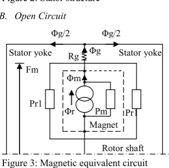
B. Open Circuit
Rotor shaft Stator yoke Stator yoke
Magnet Fm
Rg Φg
Φm
Φr Pr1
Pr1 Pm
Φg/2
Φg/2
Figure 3: Magnetic equivalent circuit
For a precise comparison with FEM results, the computation of flux density distribution is detailed in this section.
To analyse the multi-pole machine, natural equipotentials are used as to reduce the magnetic equivalent circuit to the per pole equivalent circuit. In so doing, the main flux paths can be identified and reluctances or permeances assigned to them firstly.
The equivalent circuit is of the form shown in Figure 3. Only half of the two-pole circuit is represented since the other one is a mirror-image of the half illustrated in figure 3.
The “Norton” equivalent circuit that represents each magnet consists on a flux generator in parallel with an internal leakage permeance:
m r r
B
A
(10)m m rec m
l
A
P
0
0
(11)With Am the pole area of the magnet, lm is its radial
thickness and Br is the remanent flux density. μrec is the
magnetic recoil permeability usually between 1.0 and 1.1 that can be computed as the ratio of the demagnetization curve slope and μ0 (relative permeability of air)[10]. For a
magnet arc of 55 degrees Am is estimated
l
l
g
r
A
mm
2
36
11
1
(12)The reluctance Rg is defined by:
g c g
A
g
K
R
0
(13)Where Kc [8] is the Carter factor to take into account the
slotting, Ag is the area through which the flux passes as it
crosses the airgap.
g
b
g
b
K
c1 1
5
(14)With b1 the slot opening while Ag was approximated
l
g
g
g
r
A
g.
15
.
15
2
36
11
1
(15)In equation (15) .15g was added at each of the four boundaries to make an approximate allowance for fringing.
Analytical calculation of flux leakage may be quite challenging. That gives the reason why some assisting empirical methods are utilised in the calculation [8]. Not therefore dealing with the design of the motor, for the configuration described above whereby the main flux path involves two adjacent rotor surface mounted magnets, it will suffice to consider that the rotor leakage permeance Pr1 is
typically 5-20 % of Pm0.
Practically, Pr1 can be included in modified Pm0: Pr1 is
then first normalised to Pm0, yielding
0 1 1
m r
r
P
P
p
(16)So that
)
1
(
10 1
0 r m r
m
m
P
P
P
p
P
(17)Next, the magnetic circuit may be solved by equating the magneto motive force (mmf) across the magnet to the mmf across the airgap, that is
g g m g
m r
m
R
P
P
F
(18)Yielding
m g r g
P
R
1
(19) a1a2
a3 b1
b2
b3 c1
c2
And finally
r m g
g
B
P
R
C
B
1
(20)
With
C
defined asg m
A
A
C
(21)In this motor Am=983.06 mm3; Ag=1156.54 mm3,
Bg=0.34 T. The airgap flux-density on open circuit is
[image:4.595.311.548.84.217.2]plotted in figure 4 showing a deviation with the FEM result of approximately 8.5 %.
Figure 4: Airgap flux density on open-circuit
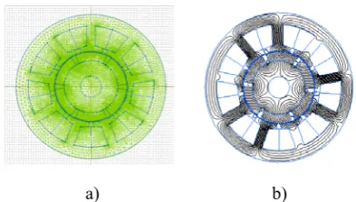
Shown in figure 5 a) and b) respectively is the meshing (triangle shape elements) of the motor generated automatically by the software and the magnetic field set up by the magnets through flux lines.
The permeability of the steel making up the stator and rotor core 1000 higher than in air is considered.
a) b)
Figure 5: a) Mesh structure b) flux lines at no-load; a rotation of 10o mechanical is captured.
C. Power Supply Structure
For the purpose of static torque computation the power supply structure is described. It is assumed that the motor is driven as in most applications [2] by a three-phase full bridge, six-pulse current converter whose the schematic diagram is presented in figure 6. It consists of 6 transistors placed in upper and lower sets, mounted back to back with a respective fly-back diode and connected to a dc voltage source V. The converter supplies power to the stator windings. The conduction period of the three phases is symmetrically phased so as to provide a three-phase set of
balance 40o (mechanical) square wave. A perfect
commutation is considered.
[image:4.595.58.242.233.350.2]A(a1,a2,a3 series) B(b1,b2,b3 series) C(c1,c2,c3 series)
Figure 6: Converter configuration
If the phases are wye connected, then at any time there are only two phases and two transistors conducting (fig. 7). Indeed, during one full electrical cycle (=2π/p mechanical; p: number of pair-poles) six different switching mode in transistor gating occur. At each moment, two transistors, one from each set (set 1-3-5 , set 2-4-6) are “on” supplying therefore two of the stator windings with opposite current waves while the third winding remains unexcited. This is schematically sketched in figure 7.
The respective transistor switching modes (#1 to #6) are shown in figure 7.
#1 #2 #3 #4 #5 #6 #1
#1 #2 #3 #4 #5 #6 #1 Figure 7: Current flow in the motor
IV. FEMCOMPUTATION RESULTS
The output torque is a quantity of utmost interest in magnetostatic analysis and is so important for performance analysis and prediction of electric motor behaviour. That torque computation is assisted here by FEA. To calculate the torque the most frequently used methods are the virtual work method, the magnetizing current method and the Maxwell stress method (MSM) [11] that is utilised in Quickfield. In the MSM the total torque will be calculated on the basis of the magnetic field distribution on a closed surface in the airgap surrounding the rotor [11]:
-0.5 -0.4 -0.3 -0.2 -0.1 0 0.1 0.2 0.3 0.4 0.5
0 100 200 300
Angle (deg.)
F
lux
de
ns
it
y
(
T
)
FEM model
V 1
0
3 5
2 4 6
A B C
iA
IB
IC
θ
θ
θ 2π/p
2π/p
2π/p
[image:4.595.328.509.408.604.2] [image:4.595.60.257.484.596.2]
rxH nB rxB nH rxn HBds T (( )( . ) ( )( . ) ( )( . )
2
1 (22)
Where r is a radius vector of the point of integration and n denotes the unit vector normal to the surface.
Unloaded and loaded machine condition were simulated in different rotor positions. The initial 0o position was
arbitrary selected in accordance with figure 5 that shows the rotor in the position 10 degrees where the top magnet is N oriented and the motor rotated counter clockwise. The similarity of the flux lines in fig. 5 b) and the ones in [9] is remarkable. In the no load instance, no current circulates the stator windings and the torque resulting from the magnetic field that is excited by the permanent magnets only is considered to assess the cogging torque of the motor (figure 8): cogging torque resulting from flux density variation around the rotor permanent magnets as they pass the non uniform geometry of the stator. It contributes to the torque ripple. On the other hand, under load simulations, the motor is supplied by ideal square waves currents having a maximum value of 2 A as depicted in the previous section.
[image:5.595.338.524.65.187.2]
The FE results show the effect of the load on the electromagnetic torque. The simulations are performed in current mode #1 when the stator is energized with chosen current steps of 0.4 up to the rated current of 2 A.
Figure 8: Variation of electromagnetic torque as a function of rotor displacement
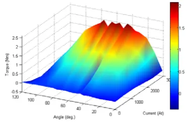
The current flows as specified in figure 7 and the torque characteristic spanned over one pole-pair pitch is presented in figure 8. From the various rotor positions and current values (0-2 A), the full torque matrix is derived and graphically illustrated in figure 9. It appears that the higher the current more significant is the torque ripple.
Figure 10 illustrates the linear dependence between the armature current circulating the stator windings and the static torque which is the average torque that the calculation will be discussed shortly, highlighting one main advantage of the PMBLDC: to retain the characteristics of a dc motor while eliminating the commutator and the brushes [4].
Figure 9: Electromagnetic torque matrix presented in 3D Finally, L. Petkovska et al [5] suggested a method to calculate the static torque that will be discussed shortly. For the authors, the fact that six times in a period (40 deg), each with Δθ=20o mech. duration, the transistor triggering is changed result in 6 pulsations function of the time of switching-on angle. So, the average value of the torque developed inside the interval Δθ for each triggering angle may be calculated from:
. 0
) , ( 1
const I
av T I d
T
(23)
[image:5.595.63.280.409.512.2]Which in our case is shown to be the middle part of the electromagnetic torque profile, i.e. the interval 50-70 deg. as shown figure 8 above and extended to interval 0-120 deg (figure 11). On fig. 11 the ideal profile of the torque free of ripple is sketched. It corresponds to a straight line.
[image:5.595.324.533.457.543.2]Figure 10: Static torque variation as a function of armature current.
Figure 11: Average torque profile -0.3
0.2 0.7 1.2 1.7 2.2
0 20 40 60 80 100 120
angle (deg.)
To
rque
(
N
m
)
Torque at 2916 At Torque at 2332.8 At Torque at 1749.6 At Torque at 1166.4 A Torque at 583.2 At Torque at 0 At
0 0.5 1 1.5 2 2.5
0 500 1000 1500 2000 2500 3000
Current (At)
Torque
(
N
m
)
0 0.5 1 1.5 2 2.5
0 20 40 60 80 100 120
Angle (deg.)
To
rq
ue
(
N
m
)
[image:5.595.335.527.600.691.2]V. DISCUSSION
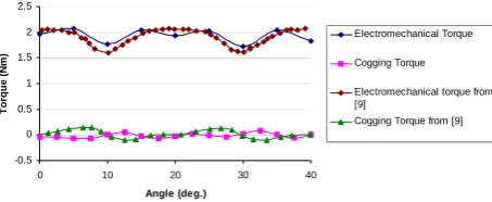
The cogging and maximum torque is computed for different positions of the rotor like in [9] specifically where the same motor has been analysed theoretically and experimentally. The procedures followed in the two latest studies differ and therefore do not enable a direct comparison between the obtained results. Nevertheless a close look at the cogging torque within the interval 0-400
[image:6.595.62.289.289.382.2]learns that the wave shapes from the current study and the one in [9] may be in opposition, they resemble. But, a discrepancy between the values is observed; the peak-to-peak cogging torque in [9] is approximately 35.6 % higher than the one in this study, i.e. 0.22 against 0.14 Nm. Those results are sketched in figure 8 that illustrates the electromechanical torque behaviour of the motor for a rotation of 400 mechanical.
Figure 12: Electromechanic torque with ideal I=2A square waves currents
Such a difference may at a certain extend be attributed to the geometric models. As a matter of fact, reproducing accurately the same geometry was quite challenging. On the other hand, in [9] a two pole section of the motor is simulated using the periodic conditions on the two boundaries and some tricks like splitting the permanent magnets in elementary pieces as to avoid numerical errors were used. Finally regarding the rated torque an error of only 2.4 % between the results is observed when the Maxwell stress tensor method is used. This tends to validate our work.
VI. CONCLUSION
Investigating the behaviour, from magnetic flux and then torque perspectives, of a PMBLDC motor was carried out in this paper. For that purpose, without resorting to any trick, the only magnetostatic analysis capability of Quick Field, a 2D FEA package was explored. The modelling of the machine was purposely detailed. As a result the flux density distribution within the machine airgap was in good agreement with the ones from the FEM. Lastly, the simulations performed on the output torque yield to results that tend to show a process successfully completed.
REFERENCES
[1] T. Wildi, Electrical machines, drives and power systems, Fith Edition, Prentice Hall, pp.571.
[2] P.C. Krause, C. Wasynczuk., D. S. Scott D, “Analysis of Electric Machinery and Drive Systems”, Second Edition, pp. 261-262, 2002. [3] W. Leonhard, control of electrc drives,3rd edition, Springer, pp,341,
201I.
[4] B. S. Ghuru, H. R. Hiziroglu, electric machinery and transfo,3rd
Edition, Oxford Press, pp. 675, 2001
[5] L. Petkovska, G. Cvetkovski, Assessment of Torques for a Permanent Magnet Brushless DC Motor Using FEA, PRZEGLĄD ELEKTROTECHNICZNY (Electrical Review), ISSN 0033-2097, R. 87 NR 12b/2011
[6] Dieter Gerling, Comparison of Different FE calculation Methods for the Electromagnetic Torque of PM Machines, NAFEMS Seminar. “Numerical Simulations of Electromechanical Systems”, Oct. 26-27, 2005, Wiesbaden, Germany.
[7] QuickField, Finite Element Analysis system V5.0, Tera Analysis Ltd, Knasterhovvej 21, DK-5700 Svendborg Denmark, pp. 188, 2012. [8] J. Pyrhonen, et al, “Design of Rotating Electrical Machines”, John
Wiley& Sons, Ltd, pp. 8, 228, 2008.
[9] N. Bianchi, “Electrical Machine Analysis using Finite Elements”, Taylor&Francis, 2005.
[10] T. J. E. Miller, Brushless Permanent-Magnet and Reluctance Motor Drive, London, U.K., Clarendon Press, 1989.
[11] A. Kostaridis,, C. Soras, V. Makios, Magnetostatic Analysis of a Brushless DC Motor Using a Two-Dimensional Partial, Computer Applications in Engineering Education, Vol. 9, no. 2, pp. 93-100, 2001.
-0.5 0 0.5 1 1.5 2 2.5
0 10 20 30 40
Angle (deg.)
Torque
(
N
m
)
Electromechanical Torque
Cogging Torque
Electromechanical torque from [9]
![Figure 1 [9]: BLDC motor structure](https://thumb-us.123doks.com/thumbv2/123dok_us/469459.545121/2.595.320.522.632.772/figure-bldc-motor-structure.webp)