Exfoliation and sensing application of 2D materials

EXFOLIATION AND SENSING

APPLICATION OF 2D MATERIALS

BY SONIA BICCAI

A THESIS SUBMITTED UNDER THE SUPERVISION OF

PROFESSOR JONATHAN N. COLEMAN

FOR THE DEGREE OF

DOCTOR OF PHILOSOPHY

IN THE SUBJECT OF

PHYSICS

SCHOOL OF PHYSICS,

TRINITY COLLEGE DUBLIN

ii

DECLARATION

I declare that this thesis has not been submitted as an exercise for a degree at this or any

other university and it is entirely my own work.

I agree to deposit this thesis in the University’s open access institutional repository or allow

the library to do so on my behalf, subject to Irish Copyright Legislation and Trinity College

Library conditions of use and acknowledgement.

Elements of this work that have been carried out jointly with others or by collaborators

have been duly acknowledged in the text wherever included.

iii

EXFOLIATION AND SENSING APPLICATION OF 2D

MATERIALS

Abstract

In the past decade, graphene and layered material such as Transition metal dichalcogenides (TMDs) and Transition metal oxides (TMOs) have been investigated for their importance in several applications. For example, these materials can be used in several fields such as energy storage and sensing device production; additionally, some of these important devices need to be scaled up for mass production. In this work, production of 2D material has been performed by liquid phase exfoliation (LPE) and the nanosheet study has been followed by strain sensor fabrication, incorporating the nanosheet in a polymeric matrix. Afterwards, a statistical computer program has been used to build a scheme able to predict the interactions between the composite variables. These predictions describe when and how the results are dependent on different variables.

Liquid phase exfoliation is a scalable method to produce large quantities of few-layer 2D materials. Here, we report on the scale-up production of WS2 in water and surfactant using shear exfoliation. Liquid exfoliation was performed changing processing parameters such as WS2 concentration, surfactant (Sodium Cholate, NaC) concentration, total volume, shear time, and shear rate. The extinction spectra for LPE WS2 was measured and empirical metrics allowed us to calculate the mean thickness and concentration of the dispersed nanosheets. The scaling equation of WS2 exfoliation in water and NaC was found and WS2 concentration and production rate were optimized, reaching a concentration of WS2 nanoflakes of 1.82 g/L and a production rate of 0.95 g/h.

iv

v

List of Keywords:

Layered Materials, 2D Nanosheets, Liquid Phase Exfoliation, Shear Mixing Exfoliation, Transition Metal Dichalcogenide, Strain Sensors, Nanocomposites, Polymers, Design of Experiment, Gauge Factor, Hysteresis.

List of

Publications

1. Khan U, Biccai S, BolandS C, Coleman J N. Low cost, high performance ultrafiltration membranes from Glass fiber-PTFE-graphene composites (in progress)

2. Biccai S, Boland C S, O'Driscoll D P, Harvey A, Gabbett C P, O'Suilleabhain D R, Griffin A J, Li Z, Young R, Coleman J N. Negative gauge factor piezoresistive composites based on polymers filled with MoS2 nanosheets. ACS nano acsnano.9b01613 (2019). doi:10.1021/acsnano.9b01613 (chapter 5).

3. Biccai S, Barwich S, Boland D, Harvey A, Hanlon D, McEvoy N, Coleman JN. Exfoliation of 2D materials by high shear mixing. 2D Materials. 2018 Oct 30;6(1):015008 (chapter 4).

4. A. J. Ryan, C. J. Kearney, N. Shen, U. Khan, A. G. Kelly, C. Probst, E. Brauchle, S. Biccai, C. D. Garciarena, V. Vega‐Mayoral, P. Loskill, S. W. Kerrigan, D. J. Kelly, K. Schenke‐Layland, J. N. Coleman, F. J. O'Brien, Adv. Mater. 2018, 30, 1706442.

vi

ACKNOWLEDGEMENT

First of all, I would like to thank Johnny for giving me the opportunity to work with him and with this wonderful group. I don’t want to get too sentimental and I’m just honest when I say that I consider myself very lucky on having him as a supervisor. He’s been a constant guide and support and thanks to him, I had the chance to grow as a scientist and overall as a person since the first Pavinar.

I would like to thank my “lab-mentor” Umar. He’s been the first one who believed that a little forgetful Sardinian chemist could go through this PhD (even before myself) and I wanted to tell him that I kept my promise and I didn’t burn and/or made explode anything. I want to thank the old Coleprople Claudia, Keith, Andrew, Dave, Damo, Tom, Peter, Victor and Zahra my liver has been trained as much as my exfoliation knowledge. I want to thank my Fitz-brothers Conor for all his support and for every “SISTER SISTEEER” sang in the lab and Dan for his incredible help and probably the craziest stories I’ve ever heard (I have just one advice for the new colemen/colewomen: don’t listen to Dan when he talks about keto-diet, it doesn’t work! case closed). To my favourite Honey Badger, to the Cowboy, and the Archangel JBriel thanks for the laughs and for brightening up the days in the office you guys made those stairs worth climbing (PS: I officially claim the ruler as mine). To Adam (the “PhD writing bible” saved this work from being just a bunch of disconnected sentences) and Seb, thanks a lot guys that key was my nightmare. To my travel partner Aideen, Yash, James and Ruiyuan for all the help, all the laughs, all the support, and overall all the drinks shared. To Ema for the coffees and the hours spent sharing the “joy” of being a PhD student. To Romina, Brigita, Patricia, my two little sisters Marta and Paola and the “new arrivals” Maria, Mia, and Dorotea thanks for putting up with me and even when every judge could have had justified an attempted murder, you just kept being my Irish family. To James (not from Donegal), thanks.

vii

mia sorella (e migliore amica) Fotokiok per esserci sempre e comunque. Ringrazio tutta la mia (non tanto normale) famiglia: tutti in un modo o nell’altro mi sostenete anche da lontano e se sono la Ponga di oggi lo devo a voi. Ringrazio la maestra Gavina e le maestre Maria Paola, Vanna e Rita per aver alimentato la mia curiosita’ da piccola, questo lavoro è un po’ anche il vostro. Un grazie speciale va a tutti i miei amici oltremare per non essersi (ancora) stancati di me: in particolare a Stefania e Iolanda spietate rivali di “cinque” e amiche insostituibili da una vita. Grazie alle mie chimiche preferite (Eli, Nini, Vale e Vero), alle mie vecchiette preferite (Eli e Gabri), al mio miramico preferito (Davide) e alle mie troddione preferite (ovviemente Giulia e Ale).

Ho concluso le precedenti tesi con una frase che in un modo o nell’altro rappresentasse il mio stato d’animo, un momento particolare della mia vita, o che semplicemente mi avesse fatto morire dalle risate e, finalmente, ho trovato quella perfetta per questo dottorato:

viii

TABLE OF CONTENTS

MOTIVATION AND THESIS OUTLINE ... 1

1.1 MOTIVATION 1 INTRODUCTION AND BACKGROUND THEORY ... 5

2.1 INTRODUCTION 5 2.2 GRAPHENE AND LAYERED MATERIALS 10 2.2.1 Transition Metal Dichalcogenides (TMDs) ... 13

2.3 EXFOLIATION OF 2D-MATERIALS 17 2.3.1 Liquid Phase Exfoliation ... 20

2.3.2 Dispersion Theory ... 23

2.3.3 Shear Mixer Theory ... 29

2.4 POLYMERS AND COMPOSITES 33 2.4.1 Polymers ... 33

2.4.2 Polyethylene Oxide (PEO)... 38

2.4.3 Polydimethylsiloxane (PDMS) ... 39

2.4.4 Composites ... 40

2.4.5 0D Particles ... 41

2.4.6 1D Particles ... 43

2.4.7 Mechanical properties of materials ... 44

2.4.8 Effect of fillers on mechanical properties ... 51

2.4.9 Effect of the fillers on the electrical properties ... 53

2.4.10 Sensing materials: Piezoresistive effect ... 58

2.5 DESIGN OF EXPERIMENT 61 MATERIALS AND METHODS ... 67

3.1 INTRODUCTION 67 3.2 MATERIALS 67 3.3 SCALED-UP PRODUCTION OF WS2 NANOSHEETS VIA SHEAR MIXING EXFOLIATION 68 3.4 COMPOSITE PREPARATION (PEO/TMDs/GRAPHENE) 69 3.5 DESIGN OF PIEZORESISTIVE MULTI-MATRIX STRAIN SENSORS (PDMS/SYLGARD/GRAPHENE) 70 3.6 CENTRIFUGATION 72 3.7 UV-VIS SPECTROSCOPY 72 3.8 RAMAN SPECTROSCOPY 75 3.9 TRANSMISSION ELECTRON MICROSCOPY (TEM) 76 3.10 SCANNING ELECTRON MICROSCOPY (SEM) 79 3.11 ATOMIC FORCE MICROSCOPY (AFM) 80 3.12 ELECTROMECHANICAL TESTING 82 EXFOLIATION OF 2D MATERIALS BY HIGH SHEAR MIXER ... 83

4.1 INTRODUCTION 83

ix

4.2.1 Pretreatment ... 85

4.2.2 Shearing step ... 86

4.3 RESULTS 87 4.3.1 Surfactant concentration variation ... 90

4.3.2 Shear rate variation ... 91

4.3.3 Initial concentration dependence ... 92

4.3.4 Volume study ... 92

4.3.5 Time dependence ... 93

4.4 CONCLUSIONS 98 NEGATIVE GAUGE FACTOR PIEZORESISTIVE NANOCOMPOSITES .... 100

5.1 INTRODUCTION 100 5.2 PROCEDURE 101 5.2.1 Nanomaterial preparation ... 101

5.2.2 Film preparation ... 101

5.2.2 Electromechanical testing ... 102

5.2.3 In-situ Raman deformation test ... 103

5.3 RESULTS 103 5.3.1 Nanosheets production and analysis ... 103

5.3.2 Composite basic characterization ... 105

5.3.3 Electromechanical properties ... 113

5.3.4 Modelling composite piezoresistance ... 117

5.4 CONCLUSIONS 124 EXPERIMENTAL DESIGN OF POLYMER:POLYMER /GRAPHENE NANOCOMPOSITES ... 126

6.1 INTRODUCTION 126 6.2 PROCEDURE 129 6.2.1 Preliminary Studies on the Variables and Program Settings ... 129

6.2.2 Sample preparation ... 133

6.2.3 Electromechanical testing ... 133

6.3 RESULTS 135 6.4 CONCLUSIONS 141 CONCLUSIONS AND FUTURE WORK ... 143

x

LIST OF FIGURES

Fig.2.1. Some of the allotropic forms of carbon ... 11

Fig.2.2. Band structure of graphene ... 13

Fig.2.3. Structure of BN, BP and TMOs ... 14

Fig.2.4. Representative structure of TMDs ... 15

Fig.2.5. Band structure of MoS2 and WS2 ... 15

Fig.2.6. Schematic of the structural polytypes of TMDs ... 16

Fig.2.7. Graphic representation of the Sol-Gel method. ... 18

Fig.2.8. Graphic demonstration of 2D-nanosheet production through CVD ... 19

Fig.2.9. Classic representation of Liquid Phase Exfoliation ... 20

Fig.2.10. Various dispersed materials obtained via LPE over the years ... 21

Fig.2.11. Examples of machines used in LPE ... 22

Fig.2.12. Schematic representation of surfactant ... 26

Fig.2.13. Representative image of the nanoparticle surface stabilised by the surfactant ... 27

Fig.2.14. Images of the shear mixer (Silverson, L5M series) ... 30

Fig.2.15. Graphic representation of shearing steps ... 31

Fig.2.16. Schematic representation of the delamination process ... 32

Fig.2.17. Different grouping of polymeric matrices ... 35

Fig.2.18. Examples of the most common plastics used and their applications ... 35

Fig.2.19. Examples of common elastomers ... 36

Fig.2.20. Schematic representation of crosslinked elastomers ... 37

Fig.2.21. Polyethylene oxide structure ... 39

Fig.2.22. PDMS structure ... 40

Fig.2.23. Schematic representation of different deformations ... 45

Fig.2.24. Schematic stress-strain diagram ... 47

Fig.2.25. Graphic representation of a plastic curve ... 48

Fig.2.26. Response of different materials as a load is applied ... 49

Fig.2.27. Schematic tensile stress-strain curve for a semicrystalline polymer ... 49

Fig.2.28. Stress-strain curve for a purely elastic material ... 50

Fig.2.29. Graphic representation of composites ... 54

Fig.2.30. Percolation steps ... 56

Fig.2.31. Schematic representation of piezoresistive behaviour ... 58

Fig.2.32. First step of DOE ... 62

Fig.2.33. Computed table of DOE runs ... 63

Fig.2.34. Data collection of DOE ... 64

Fig.2.35. Display of model specification to fit the data of DOE... 65

Fig.2.36. Prediction profiler of an experiment designed ... 66

Fig.3.1. Extinction, Absorption and scattering spectra of MoS2 ... 74

Fig.3.2. Graphic representation of Rayleigh and Raman scattering. ... 76

Fig.3.3. Schematic of a TEM column ... 78

xi

Fig.3.5. Schematic representation of a SEM column ... 80

Fig.3.6. General representation of AFM operation ... 81

Fig.3.7. Schematic representation of tensile tester apparatus...83

Fig.4.1. Graphic representation of WS2 preparation... 85

Fig.4.2. Images of impurities collected after pretreatment ... 85

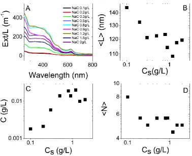
Fig.4.3. Extinction coefficient vs ratio of extinctions at A exciton and at 350 nm 88 Fig.4.4. Ratio of extinction at 365 nm and 465 nm vs flake size ... 89

Fig.4.5. TEM images and relative histogram and Raman spectrum of WS2 in H2O/NaC ... 90

Fig.4.6. UV-vis spectra, C, <L> and <N> of WS2 vs NaC concentration ... 91

Fig.4.7. AFM and concentration of WS2 vs processing parameters ... 94

Fig.4.8. WS2nanosheets’ thickness as a function of processing parameters. ... 95

Fig.4.9. WS2 nanosheets’ length as a function of processing parameters ... 96

Fig.4.10. UV-vis spectrum of WS2 at high concentration ... 97

Fig.4.11. WS2 concentration versus scaling equation with high concentration value ... 97

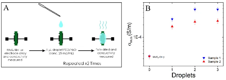
Fig.5.1. Nanocomposite films containing different MoS2’s loading level ... 102

Fig.5.2. Characterizations of MoS2 dispersion ... 104

Fig.5.3. TEM of WS2, MoSe2, WSe2 and graphene nanosheets ... 105

Fig.5.4. Raman spectra measured on a PEO film and MoS2/PEO. ... 106

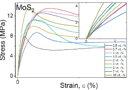
Fig.5.5. Stress-strain curves of different MoS2 mass fractions ... 107

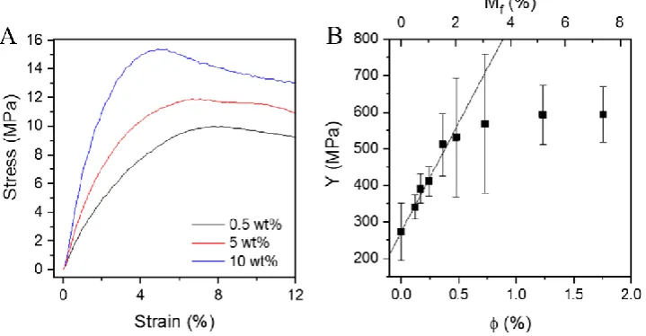
Fig.5.6. Representative stress-strain curves for selected MoS2/PEO composites 108 Fig.5.7. Conductivity plotted versus MoS2 volume fraction for MoS2/PEO composites. ... 111

Fig.5.8. The procedure adopted in order to verify the doping effects of PEO on MoS2 ... 112

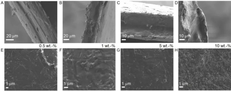
Fig.5.9. SEM images of composite PEO/MoS2 films for different Mf. ... 113

Fig.5.10. Electromechanical response of MoS2/PEO ... 114

Fig.5.11. Raman band position vs strain ... 115

Fig.5.12. Dynamic strain profiles vs resistance at three different frequencies ... 116

Fig.5.13. Response of 5wt.-% MoS2/PEO composite to step strains ... 117

Fig.5.14. Resistance vs strain plot for two samples of PEO/graphene samples. . 121

Fig.5.15. RJ,0/RNS,0 vs ϕ. ... 122

Fig.5.16. Typical stress/strain and resistance/strain curves of PEO composites. ... 124

Fig.5.17. Representative resistance-strain curves for composites of PEO ... 124

Fig.6.1. Polycondensation reaction of PDMS ... 126

Fig.6.2. Stress-strain curve of G-Putty and its hysteresis value (inset). ... 127

Fig.6.3. n! relationship between variables and samples required ... 128

Fig.6.4. Gauge factor as a function of time at 50, 70 and 100 °C ... 130

xii

Fig.6.6. Stress-strain curve of a viscoelastic material during a loading-unloading

cycle. ... 134

Fig.6.7. Stress-strain curves with calculated hysteresis (inset) for each sample prepared. ... 135

Fig.6.8. ΔR/R0, as a function of strain ... 136

Fig.6.9. Table of DOE with reported results ... 136

Fig.6.10. Prediction profiler with a selection of random factors ... 137

Fig.6.11. Stress-strain curve and ΔR/R0 as a function of strain % of the DOE. .. 138

Fig.6.12. Prediction profiler of the best sample ... 138

Fig.6.13. Images of the final nanocomposite ... 139

Fig.6.14. Dynamic strain profiles at two different frequencies ... 139

Fig.6.15. Responses of Sylgard/PDMS/graphene composite to step strains of 4%. ... 140

xiii

LIST OF TABLES

Table 3.1. DOE test 63

Table 4.1. Pretreatment parameters 75

Table 4.2. Shearing parameters 76

Table 4.3. Beakers capacitance 81

Table 6.1. Sylgard curing times vs temperature 108

xiv

To Dario,

For the best puzzle

competitions I have ever had

To my Nonno,

For the best “pani e zuccaru”

I could ever wish

1

1

Motivation and Thesis Outline

1.1 MOTIVATION

Throughout the past decades, nanoscience has been the driving force towards technological progress while over the last 15 years, an enormous jump forward has been made thanks to the joint findings of chemistry, engineering, and material science. When the first carbon nanotubes1,2 and fullerenes3 were described, the interest of industry was brought towards nanomaterials; however, it was only after the isolation of graphene4 in 2004, and the successful re-discovery of layered materials,5–8 that this interest grew exponentially. There has been plenty of confident speculation over the potential of these materials, and, in order to fully harness this potential, a separate branch of material science has been developed. This new branch has been dedicated entirely to the preparation, scalability, and application of layered materials.9–17

2

NaC) and developed an equation that describes the WS2 final concentration as a function of several parameters.30

This brought us to the second part of our work where TMDs have been incorporated in a polymeric matrix for sensing applications. Indeed, while other more conducting materials have been widely explored, TMDs based strain sensors are not commonly investigated because of their lower conductivity. Furthermore, a model that describes the piezoresistivity of polyethylene oxide (PEO) nanocomposites has been developed, which focused our attention on negative piezoresistivity of PEO/molybdenum disulphide (MoS2) composites. Finally, we went from a simple system of strain sensor composed of just a polymer (PEO) and filler (TMD) to a more complex system where nanocomposites have been prepared using exfoliated graphene as a filler and a mixture of two different polymers as a matrix. Several variables have been changed with the purpose of enhancing the sensors’ electromechanical properties by combining mechanical properties of both polymers and conducting characteristics of graphene. For this reason, a statistical program (Design of Experiment, DOE) has been used to “design the experiment” by finding the optimum combination of the variables involved.31,32

Furthermore, using a prediction profiler of the aforementioned program, it was possible to define the relationship between the variables used in the experiment and improve the responses important in sensing materials such as hysteresis and gauge factor. Through our endeavour to model these dispersions, reviewing the main findings in sensing applications, and profiling complex polymeric systems through statistical analysis, it is hoped that this work will provide a richer picture of TMDs’ characteristics and piezoresistive materials for future developments.

1.2 THESIS OUTLINE

Chapter 2 – Introduction and Background Theory

3

the Young’s modulus definition to piezoresistivity description are explained. Finally, a brief summary about the design of experiment and the principles that brought on the development of this concept is described.

Chapter 3 – Materials and Methods

The chapter comprises the materials, the sample preparation process and the characterization used during the course of this work. A brief description of the equipment used during electromechanical testing is also presented.

Chapter 4 – WS2 Exfoliation via High Shear Mixing

In this chapter, shear mixer exfoliation is explained, results are reported of the experiments conducted, and the technique to create a scale-up equation that can describe the efficiency of this preparation method, is presented.

Chapter 5 – Negative piezoresistivity of PEO/MoS2 nanocomposites

In this part of the thesis, the technique of how TMDs are prepared via liquid phase exfoliation is presented. These particular TMDs are introduced into a polymeric matrix and the resulting composite is used for strain sensing applications. We focus our attention on molybdenum disulphide and polyethylene oxide. Here, the polymer acts as a dopant, increasing the conductivity of MoS2. Furthermore, it is shown how the stress is transferred into MoS2 nanosheets at small strain, modifying the band gap and giving them the characteristic negative gauge factor. Lastly, a model has been developed to describe all these observations and we compare several materials including tungsten disulphide, molybdenum diselenide (MoSe2), tungsten diselenide (WSe2), and graphene.

Chapter 6 – Experimental Design (DOE)

4

obtain high elastic strain sensor performances (i.e. low hysteresis and high gauge factor).

Chapter 7 – Conclusions and Future Work

5

2

Introduction and Background Theory

2.1 INTRODUCTION

6

photoluminescence) to the material useful for applications such as batteries24,45,55 or sensors55–57 and some of these important applications will demand industrial-scale production.20 For this reason, it is important to find a method which leads us to large scale, defect free production of 2D nanomaterials (i.e. without oxidation reactions). Regarding mechanical properties, the AFM analysis of MoS2 with the number of nanosheets between 5 and 25, shows high Young’s modulus (0.33± 0.07 TPa) and 1 or 2 layers of MoS2 have been found broken, but highly crystalline and defect-free.50 _{Due to its excellent semiconducting properties, single-layer MoS}

2 nanosheets are suitable for a variety of applications such as flexible electronic devices.34,58,59 Furthermore, the thickness dependent band gap of MoS2 nanosheets is seen as an important characteristic that can be exploited for optoelectronic devices.60 Thanks to the space between the S-W-S sheets, WS2 is an excellent candidate for intercalation reactions and, therefore, for high energy density battery production.45 Moreover, the performances of single and bilayer WS2 transistors have been studied, finding their electronic transport properties interesting and suitable for this kind of application.61

Despite their properties, these materials are not widely used because most of their exfoliation methods are not scalable (i.e. scotch tape method; Chemical Vapour Deposition (CVD)). Applying these methods, it is possible to obtain material with a good yield and crystallinity, but it is not possible to scale these methods up for industrial quantities. A more suitable method that can lead to the achievement of a large amount of nanomaterial is liquid phase exfoliation (LPE).62

LPE is an efficient technique for dispersion and exfoliation of several layered nanomaterials. It is a top down method where a layered material is immersed in a liquid, a solvent or aqueous surfactant, then, ultrasonic agitation supplies energy for cleaving the layers of the material.18 Liquid exfoliation through sonication gives defect-free nanosheets, but the scalability of this process is restricted by the low yield and the high amount of energy this technique requires. One possible alternative to sonication would be high-shear mixing.

7

This work shows successful implementation of a technique to exfoliate massive quantities of defect-free WS2 (Chapter 4); this technique is known as shear mixing exfoliation. As the name suggests, the exfoliation occurs by shearing the 2D materials via two main parts: a four blade rotor and a stator. We demonstrate that the theory describing shear exfoliation of 2D materials in the liquid phase can be applied not just to graphene as previously reported, but also to other materials. In this work we focus our attention on one material of interest (WS2) and, through varying processing parameters, demonstrate that scalable production of WS2 can in fact be performed using high shear mixing.30

Even though research in liquid exfoliation has a lot to offer, our work was not solely intended to focus on the shear exfoliation of TMDs, rather it wanted to be pushed towards the application work, specifically, on strain sensors (Chapter 5).

8

/

R R G

 

(1.1a)

where G is the gauge factor and ε is the strain applied. Usually, the gauge factor is measured at low strain and in that limit it can be shown that68

0

1 d

(1 2 ) d

G  

 

  

(1.1b)

9

interaction at the Ru//AlN interface has an effect on the value of the piezoelectric response.89 In addition, SiC, Ge and GaAs also have reasonably high negative values of G.82 However, most interestingly for this work is the fact that the band gap of the 2-dimensional semiconductor MoS2 (i.e. the 2H polytype) tends to fall with strain,90,91 _{leading to negative gauge factors ranging from –225 for bilayer} MoS2, to –50 for few-layer MoS2.58,92 To the best of our knowledge, no composites of polymers filled with semiconducting particles have been reported with negative G for two main reasons. Firstly, due to the low conductivity that a polymer filled with semiconductors implies. Secondly, even if such studies were made using negative piezoresistive particles, it is difficult to transfer an applied strain to the filler particles. Consequently, applied strain causes the motion of the adjacent fillers, rather than deforming the particles; while, the particle deformation would change the band gap and reduce the particle resistance.93

10

polydimethylsiloxane (PDMS)107,108 or polyurethanes (PU).109,110 A problem with these types of strain sensors is the filler cracking, which occurs after several cycles, and the consequent detaching from the substrate. Another option that would avoid this problem is preparing strain sensors where the conductive filler (or conductive polymer) is embedded within a polymer matrix;111–116 _{here it is possible to combine} and control the properties (mechanical and electrical) of both polymer and filler but it is necessary to consider the interactions between these two in order to optimise their characteristics and obtain high gauge factor and low hysteresis. However, this has been challenging to achieve and a way to do so is combining more than two components. In this way, we can create a complex system that can be modulated in order to obtain the expected results. Nonetheless, more variables imply also more testing to perform thus, more time and money to spend on the experiment. One solution could be the use of Design of Experiment or experimental design (DOE).117–119 Design of experiment is a method which harnesses statistical calculation regarding a specific experiment in order to predict the best results achievable from that experiment.120 With this method it is possible to predict the desired results (called “responses”) of an experiment through statistical analyses. In order to use this method in the most appropriate way, we need a pre-phase. Here, the variables necessary to perform the experiment (referred to as “factors”) are defined and a specific range of values of the variables is specified in the program. This technique, commonly used in industries, represents an efficient way to perform every kind of experiment in a broad range of fields; from the realization of chemical reactions,121,122 _{to the optimization of devices used in renewable energy}123–128 _{or to} improve biomedical materials’ performances.129–132

2.2 GRAPHENE AND LAYERED MATERIALS

11

properties to the single-layer one.4,18,133 However, graphene is an allotropic form of carbon as well as fullerenes (hexagonal and pentagonal units connected together in a spherical shape)2 and carbon nanotubes (graphene sheet wrapped to form a tube)39,84,93 (Fig.2.1). Graphene has exceptional properties, including: high value of Young's Modulus close to that of diamond, high breaking strength, high specific surface area, and very high thermal and electrical conductivity.33,41 Electrons can move in the graphene lattice without encountering obstacles and this allows for a much higher mobility than the one present in metals or semiconductors (Fig.2.2).134 Thanks to these properties, the potential applications are innumerable; some applications are: energy storage,135 electronics, production of transistors components and microchips,28 optics,33,47 biomedicine16,70 and production of nanocomposite materials,136–138 the latter of which aligns most closely to our interests.

12

13

Fig.2.2. Band structure in the honeycomb structure of graphene. We can see the that the energy at the Dirac points is zero and because it is gapless, graphene is

considered a semi-metal.134

2.2.1 Transition Metal Dichalcogenides (TMDs)

14

consequently, some diverse properties.144 Usually used for their catalytic activity and their semiconductive properties, TMOs can be used in photo-assisted processes145–147 or electronic devices.148–150

Fig.2.3. Structure of a) Boron Nitride,151 b) Black Phosphorus152 and c) some examples of Transition Metal Oxide compounds (MoO3 on the left and V2O5 on the

right).153

15

Fig.2.4. Representative structure of TMDs.159

The band structure for these compounds changes drastically going from the indirect gap in bulk samples to the direct gap in single layer nanosheets (Fig.2.5).160 _This affects the electrical and optical properties which depend on the numbers of layers, especially for samples with less than five layers.155

Fig.2.5. Band structure of both MoS2 (on the left) and WS2 (on the right) from

16

Their electrical properties are very sensitive to external factors such as temperature, strain and pressure.161 Moreover, the presence of defects in the form of vacancies, adatoms and boundaries can lead to fascinating magnetic properties.58,61,157 There are about sixty TMDs where just a third does not have layered structure,162 mostly are synthetic but, a good portion exists in nature such as MoS2 in its forms 2H and 3R (here the numbers represent the number of layers in the unit cell of the compound and the letters H and R specify the symmetry, i.e. H = hexagonal, R = rhombohedral, T = trigonal, Fig.2.6). These polymorphs can be stacked or arranged in 3 different polytypes.162

Fig.2.6. Schematic of the structural polytypes of TMDs from left to right 1T (tetragonal symmetry with octahedral coordination of the metal and one repetition of the layer), 2H (hexagonal symmetry with trigonal prismatic coordination of the metal and two repetition of the layer), 3R (rhombohedral symmetry with trigonal prismatic coordination of the metal and three layers per

repeat).

17

respectively.10,11,48,163 Previous work done by Backes et al., relates qualitatively and quantitatively the extinction spectra to specifically the MoS248 and WS211 length and thickness, developing metrics for these materials exfoliated via liquid phase exfoliation. Indeed, the atoms at the edges of the flakes have different effects on the local absorption coefficient, thus the optical absorption. When the length of the nanosheet is reduced, the ratio of edge to central atoms increases, causing a change of the spectral shape. Regarding the thickness of the material, it has been previously demonstrated that if we reduce the number of layers, we confine the electrons into a 2D space; this change can be observed in the optical spectrum through the shifting of A-exciton (defined as electrically neutral quasiparticle commonly presents in semiconductors which is able to transport energy without a charge transport) as well as the extinction spectra.10,11,17,19,48

2.3 EXFOLIATION OF 2D-MATERIALS

Over the years since 2004, several synthesis approaches have been developed with the purpose of improving both processing quality and quantity of 2D nanosheets.24,33,158,164,165 These methods can be broadly classified into bottom-up or top-down, depending on how the monolayer is obtained. Briefly, the starting materials of the bottom-up approach are atoms and molecules which self-assemble into building blocks and subsequently into a nanostructure through physical and chemical interactions;166,167 one example is the Sol-Gel method (fig.2.7). This technique is generally used to prepare 2D materials, in particular metal oxides, as well as oxide composites.168–173 The Sol-Gel method is a wet-chemical process where the metal precursor of the nanoparticles is immersed in a liquid forming colloidal suspension (Sol) first and subjected to a gelation process afterwards (Gel).174 This method comprises few steps before obtaining the final product:

- Hydrolysis step (fig.2.7a). Here, the formation of metal hydroxide occurs. - Condensation step (fig.2.7b). A condensation reaction leads to a gel

18

- Drying process (fig.2.7c). In this step the final product can be obtained through evaporative drying (forming a Xerogel), or through supercritical drying (forming an Aerogel).174

Moreover, the Sol-Gel can be divided into two categories; aqueous Sol-Gel172,173,175 which consists of the use of water as solvent and non-aqueous Sol-Gel, where an organic solvent replaces water as solvent.176 _{In several cases, especially for the} aqueous Sol-Gel, the key steps of hydrolysis, condensation, and drying process take place at the same time causing a difficult morphology control and repeatability of the protocol.168,170,171

Fig.2.7. Graphic representation of the Sol-Gel method.

19

The copper layers are subsequently evaporated, leaving a single layer of graphene on the surface of the dielectric material.164,177 It has been successfully demonstrated that it is also possible to obtain TMD nanosheets using a slightly different synthesis method. Indeed, instead of hydrocarbons, this process involves heating a metal oxide precursor (Fig.2.7).178 _{Chemical methods offer the advantage of control over} both nanosheet size and thickness, creating good quality monolayers; however high-yield electronic device production requires an alternative method of production which is more scalable than CVD or Sol-Gel.

Fig.2.8. Graphic demonstration of 2D-nanosheet production through chemical vapour deposition (CVD).179

20

mechanical energy overcomes the weak Van der Waals forces between the layers. Despite the fact this method enables the production of high quality monolayers, the method has a very low yield which means scalability is not a possibility.4

2.3.1 Liquid Phase Exfoliation

The need to find an ideal method that can lead to both high quality nanomaterials with the ability to control their size, thickness, flake orientation, as well as an easy and cheap processing technique, has been the main objective of research in this field. For the scope of this work (which aims to use 2D-materials in electronic devices), it is very important to find a method that comprises all these features. In fact, the presence of defects in the material can affect the electric properties (i.e. conductivity) resulting, consequently, in poor performances of the electronic device. However, none of the techniques developed to-date have been able to combine all these characteristics; nevertheless, the possibility of high yield and high quality nanosheets have made the liquid phase exfoliation process very appealing in the 2D research world. This liquid phase exfoliation (LPE) process was demonstrated for the first time in 2008 by Hernandez et al.,18 when the achievement of exfoliated graphene from graphite through ultrasonication was shown (Fig.2.8). The graphite powder was dispersed into a specific solvent (N-methyl pyrrolidone) to prevent the reformation of the hydrogen/Van der Waals bond once exfoliated, and thus, reaggregation of the nanosheets.18

21

In the paper mentioned above,18 it was shown how it is possible to harness nanosheet-solvent thermodynamics (section 2.3.2) to achieve high yield and quality of the exfoliated material. This technique is extremely versatile and since its first use, it has progressed significantly to exfoliate other layered materials such as TMDs, TMOs, hBN, BP, hydroxides (Fig.2.9), etc.19

Fig.2.10. Various dispersed materials obtained via LPE over the years.19

22

Fig.2.11. Examples of machines used in LPE: a) sonic bath, b) sonic tip, c) kitchen blender and d) shear mixer.

23

2.3.2 Dispersion Theory

As previously mentioned, a careful choice of solvent (or surfactant in the case of aqueous dispersions) is necessary to obtain a good dispersion where the material is not just exfoliated but also stable in the liquid medium without reaggregation. To achieve this, a theory that describes both the physics and the chemistry behind the liquid exfoliation process has been developed from Coleman’s work.18,193 _The dispersion theory is a fundamental part of liquid phase exfoliation, and it can be divided into two methods: one method considers the exfoliation through a solvent (Solvent Exfoliation Mechanism), and the other method studies the mechanism of the process using water/surfactant (Electrostatic Stabilising Mechanism or Surfactant Exfoliation). These two methods are analogous, and in this thesis, both methodologies are described.

Solvent Exfoliation. The stability of a solute in a solvent depends on two factors: the type of the solute and the nature of the solvent. In fact, nanomaterials with a certain structure can have different chemical interactions depending on the surrounding environment. In the case of TMDs, graphene or other layered materials, the forces responsible for their interlayer bonding are the Van der Waals dispersive forces. A theory developed by Hildebrand194 and later developed by Hansen,195 demonstrated that by matching Hildebrand solubility parameters of the solvent and the solute, it was possible to obtain a stable dispersion of the nanomaterial. Strictly speaking, we can assume (from Hamaker theory) that solute and solvent with similar surface energy gives a stable dispersion196_{. Therefore, the} interaction can be described very simply by analysing the Gibbs free energy of the mixture and, for ideal dispersions, ΔGmix has negative values. This quantity is the combination of two factors: the enthalpy of mixing and the mixing entropy and is defined as

mix mix mix

G

H

T S

24

Here, T is the temperature, ΔHmix is the enthalpy of mixing, and ΔSmix is the entropy of mixing. For a negative ΔGmix, we need to minimize ΔHmix; thus it is necessary to consider and include other important parameters. In fact, it is not sufficient to describe just solute-solvent interactions, but also solvent-solvent and solute-solute interactions. It is even possible to achieve a better understanding by applying the Flory-Huggins theory.193 In this case, ΔHmix can be described by:

0

(1

)

/

mix

H





kT









Here, φ is the solute volume fraction, ν0 is the volume of one molecule and χ is the Flory-Huggins parameter. This parameter χ is defined as:

(2

)

2

AB AA BB

z

kT









 





Here, z is the coordination number of both solvent and solute and ε represents the inter-molecular pairwise interactions.

Looking at the equations (2.2) and (2.3), we notice several things. First of all, we have to take solute-solute and solvent-solvent interactions into account, not just solute-solvent interactions (represented in the equation (2.3) by A and B). Second, solute-solvent interactions are dominant if χ<0 while if χ>0, the solute molecules are attracted to each other causing aggregation of the nanosheets. This also means that the smaller χ is, the smaller ΔHmix will be and, consequently, will promote a better dispersion.193

25

dispersive energy (ED), polar cohesive energy (EP) and the electron exchange parameter (EH). The total sum of these parameters is the total cohesive energy (E),

D P H

E



E



E



E

The Hildebrand parameter is the sum of the squares of each Hansen parameter ( /

E V

  , where V is the molecular volume).

2 2 2

2

D P H















Thus, it is possible to express χ in terms of Hansen parameter:



 

 



0

, , , , , ,

D A D B P A P B H A H B

kT





































By matching Hansen parameters of solutes and solvents, it is possible to minimise (δA- δB)2 and, consequently, minimise the mixing enthalpy encouraging dispersion stabilisation.193–195

26

Fig.2.12. Schematic representation of (a) surfactant and (b) sodium cholate molecule used in this work.

Therefore, in LPE the hydrophobic tail will be attracted to the nanoparticle while the polar phase is solvated by the water. The most commonly used surfactants used in LPE are ionic compounds such as sodium cholate (SC or sometimes NaC,

27

Fig.2.13. Representative image of the nanoparticle surface (grey) stabilised by the surfactant (pink).

This charge distribution around the nanoparticle produces a potential difference (electric double layer, EDL)198 which can be described by the DLVO theory; the theory takes its name from people who studied this phenomenon (Derjaguin, Landau, Verwey, and Overbeek). DLVO theory assumes that for dispersed spherical particles with an equilibrium of attractive and repulsive potential energies, the attractive energies depend on Van der Waals weak bonds and the repulsive forces are influenced by the EDL. Consequently, to have a dispersion of the nanoparticles the EDL has to be greater than VdW forces. It is possible to describe this mechanism through the equation:

A R

28

where the total potential energy, V, is the sum of attractive, VA, and repulsive, VR, potential energy. VA for two spheres in vacuum, with radius r, at distance D can be expressed by

12

Ar

V

D

 

where A is the Hamaker constant.196

VR can be described by several factors. It depends not just on the size and the shape of the nanoparticles but also on the distance between them, and on the Zeta potential, ζ, which is the key indicator of the stability of a colloidal dispersion. The magnitude defines the potential at the nanoparticle surface and it indicates their repulsion degree. Moreover, VR depends also on the dielectric constant of the liquid, 𝜀_𝑟, and the Debye screening length, 𝜅−1_{, which represents the effective thickness}

of the EDL199

1/ 2 1 0 2 0

2

kT

e n

 



 











where ε0 is the permittivity of free space and n0 is the concentration of the surfactant. For two small particles with radius r when κr << 1 then

2 2 0 D r R

r

V

e

D

  



29

12

r

Ar

V

e

D

D

  

 



(2.11)

From the equation above, we can say that the Zeta value has to be high in order to avoid reaggregation, typically around 30mV. Even though this model describes the potential for two spherical nanoparticles without considering the orientation effects or planar objects, it gives an idea of the mechanism and physical parameters involved in this process.

2.3.3 Shear Mixer Theory

30

Fig.2.14. Images of the shear mixer (Silverson, L5M series), working head (top) and the different stationary phases (bottom).212

During the rotation, the shear mixer acts as a pump. It is possible to describe the whole process in four stages (fig.2.14):209

31

- The material horizontally ejected from the workhead is led to the edge of the mixing vessel and, at the same time, fresh material is drawn into the workhead maintaining the mixing cycle.210

Fig.2.15. Graphic representation of shearing steps.

An important parameter to consider is the shear rate, one of the values which are related to the exfoliated material.213 The approximate shear rate (𝛾̇) can be calculated via the following equation:

ND

R









where N is the rotation per second, D is the diameter of the shear head and ΔR is the gap between rotor and stator (~100 μm).214,215

32

force applied induces a partial sliding, and finally, we have complete delamination of the flakes.20,209,216

Fig.2.16. Schematic representation of the delamination process in terms of interfacial energies.20,217

It is also possible to analyse the delamination process in terms of interfacial energies and as described from Paton K. et al;20 the energy change on the delamination process can be estimated (using the geometric mean approximation E_LP  E E_{LL PP}

) by the following formula:

2 2

LL PP

E

L



E

E



 







where ELL is the interfacial energy associated with Liquid-Liquid interaction, EPP is related to the Platelet-Platelet interaction and ELP (fig.2.15) is correlated to the Liquid-Platelet interface. Furthermore, the minimum applied force for delamination (Fmin) can be obtained from the derivation of the energy: (−𝜕𝐸(𝑥)/𝜕𝑥). Moreover, using the geometric mean approximation (ΔE>0) we have20

2

min LL PP

33

Consequently, we can define the minimum shear rate to exfoliate particles with L size by20

2

min

LL PP

E E

L





  

 

 (2.15)

2.4 POLYMERS AND COMPOSITES

2.4.1 Polymers

A polymer is a chemical compound defined as a macromolecule, or large molecule, which is composed of a high number of repeated subunits.218 Due to their broad range of properties, there are different ways to classify polymeric materials (fig.2.17); from categorizing polymers depending on their molecular characteristics (fig.2.17 a), to the type or polymerization reaction (fig.2.17 b) or the source type from which these polymers are fabricated (fig.2.17 d). Another way is according to their end-use and, depending on its properties, a particular polymer can be used in more than one application. For the purpose of this work, which aims at the use of composite as strain sensors, the last classification has been selected to describe the different characteristics of polymers at first and composites afterwards (emphasizing the attention on the mechanical and electrical response). The various types of polymers include plastics, elastomers (or rubbers), miscellaneous (fibres, coatings adhesives, foams, and films) and advanced materials which include thermoplastic elastomers, liquid crystal polymers, ultrahigh molecular weight polyethylene (UHMWPE).219 Ultrahigh molecular weight polyethylene

34

35

Fig.2.17. Different grouping of polymeric matrices based on a) the molecular characteristics, b) the response at high temperature, c) the polymerization

reaction and d) the source.220

PLASTICS

Plastics is a general term to define synthetic or semi-synthetic organic polymers most commonly derived from petrochemicals. It is possible to classify their mechanical properties between elastomers and fibres.222 _{Polymers belonging to this} category may have different degrees of crystallinity, molecular structure or configuration, which implies that some are very flexible and can exhibit both elasticity and plasticity while some of them are rigid and brittle (fig.2.18).222,223 Moreover, they can be thermosetting or thermoplastics depending on their molecular features. However, we can define a polymer as plastic when they maintain their shape below their glass temperature (if amorphous), below their melting temperature (if semi-crystalline) or when crosslinked. Numerous plastics reveal exceptional properties, such as optical transparency (PS, PMMA), chemical attack resistance (Teflon), mechanical strength (Nylon)220,221,224 and, for this reason, they are used in countless applications (e.g. lenses, coatings, bearings, gears, safety helmets, toys, bottles, pipes, etc).

36

ELASTOMERS

One of the most fascinating properties of elastomers is their ability to be largely deformed and spring back to their original form when they are in an unstressed state. The elastomeric behaviour, due to crosslinks between the chains, was first observed in natural rubber (Fig.2.19).182

Fig.2.19. Examples of common elastomers.220

37

Fig.2.20. Schematic representation of crosslinked elastomers in both relaxed and stressed mode on the left, and stress-strain behaviour for brittle (a), plastic (b),

and elastic (c) materials on the right.

MISCELLANEOUS APPLICATIONS

- Fibres. The most common fibre polymers are use in the textile industry; they typically have a 100:1 length/diameter ratio. While in use, fibres may be subjected to a variety of mechanical deformations such as shearing, twisting, stretching and abrasion. Therefore, they must have high tensile strength and high elasticity modulus, as well as abrasion resistance. These properties depend on both chemistry of the polymer chains and the fabrication process.

38

penetrates into the pores of the surface attached (i.e. methacrylates).226 Chemical bonding comprises both covalent and weak bonds (i.e. Van der Waals) between the adhesive and the adhered material; in the case of VdW bonds, polar functional groups enhance the adhesion. Depending on the type of the surface on which to adhere, a selective polymer can be used. Albeit different natural polymers have adherence characteristics (casein, starch, animal glue), synthetic polymers such as polyurethanes, polysiloxanes (silicones) and acrylates are commonly used as adhesives.182,220,226

- Foams. Foams can be defined as plastic materials with a high percentage in volume of bubbles trapped in the solid matrix. This type of polymer is commonly used in thermal insulation as well as packaging and furniture. Typical materials belonging to this class are polyurethanes, rubbers, polystyrenes and PVC.

- Films. Films are polymeric materials with a thickness between 0.025 and 0.125 mm. These compounds are fabricated for several purposes among which there are food packaging, textile products, and in the last decade for biomedical uses.220 _{These materials are characterised by a high degree of} flexibility, high tensile strength and high tear strength. In this work, Polyethylene oxide (PEO) films (as well as PDMS films) have been fabricated with the purpose of finding a biocompatible and flexible material for sensing applications.

2.4.2 Polyethylene Oxide (PEO)

39

chemical and biological fields, this polymer is categorized as a function of its molecular weight. For this reason, PEO is considered as such if its molecular weight is above 20,000 g/mol.

Fig.2.21. Polyethylene oxide structure.

The PEO at room temperature is tough, exceptionally crystalline, and it shows a moderate Young’s modulus that changes proportionally with its molecular weight. Moreover, it has very high elongation, and it is characterized by the ability to orient when stressed. Although PEO is water soluble, its tensile properties are not significantly affected by the humidity up to 90%, where it drops drastically.227 Furthermore, PEO can be processed using the methods for common thermoplastic polymers such as molding, extrusion, etc.182 _{Usually, this polymer is used as an} additive or, most commonly, as a component for copolymer preparation combining the properties of two or more matrices and subsequently used in several applications ranging from biomedical to high-performance battery fabrication.229–231

2.4.3 Polydimethylsiloxane (PDMS)

40

Siloxanes comprise a backbone of alternating silicon-oxygen repeating units with organic chains attached to the silicon atoms, in the case of the PDMS, as the name suggests, the organic chains attached are two methyl groups (Fig.2.22).

Fig.2.22. PDMS structure.

Thanks to long and highly flexible backbone chains, PDMS has rubber-like properties. This polymer is classified as a viscoelastic, non-crystalline elastomer and depending on the type and the degree of crosslinking we have different mechanical responses (i.e. physical crosslinking for silly putty,137,138 and chemical crosslinking for Sylgard 170®234). The presence of methyl groups gives the high hydrophobicity to the molecule as a consequence, in case of chemical crosslinking, non-polar solvents (THF, chloroform) are able to swell considerably this polymer. Also, depending on the demand, the properties of this polymer can be easily tuned finding place in several applications from contact lenses and medical devices235–237 to shampoos238 and anti-foaming agent.239–241

2.4.4 Composites

41

a filler or reinforcement. The matrix comprises a continuous homogeneous phase which encloses the reinforcement (called also filler) and ensures that the particles of the latter are dispersed inside the composite without segregation. Thus, depending on the type of composite we want to obtain, the choice of the matrix is important as much as the filler choice.

The reinforcement (or filler) constitutes the dispersed phase in the matrix and we can classify composites based on the type of reinforcement in 1) particulate composites, 2) fibre reinforced composites (continuous and discontinuous), and 3) structured composites (formation of interpenetrating lattices). Particular composites consist of particulates dispersed in the matrix (e.g. gravels, micro-granules, and resin powders). The latter has a marked anisotropy (a property for which a given object has characteristics that depend on the direction along which they are considered).224 In both cases, there is no significant interaction between the matrix and reinforcement interface, but in the case of the fillers, if the filler is on the order of nanometres, the so-called nano effect220 takes place. This effect is defined by an increase in surface atoms and, consequently, the interfacial region rises considerably. In this case we can define a nanofiller as a reinforcement. This type of filler leads to a very high contact area between matrix and filler and therefore to a significant increment in a variety of performances. Based on the dimensions (length, width, height) of the dispersed particles, we can classify the nanofillers into isodimensional particles (0D), when the three particle sizes are of the order of nanometres (i.e. fullerenes, POSS, metals);243,244 one-dimensional particles (1D), such as nanotubes or whiskers, when two dimensions out of three are nanometric;182,245 _{two-dimensional (2D) particles, when only one dimension in} three is nanometric (TMDs, TMOs, graphene). In this case, the filling material is present in the form of sheets with a thickness of a few nanometres.

0D and 1D particles are described more in depth in the two paragraphs below, whereas 2D materials, such as graphene and TMDs, and their characteristics have been previously described (section 2.2).

42

As mentioned above, POSS, fullerenes and metals are isodimensional particles examples.

POSS (polyhedral oligomeric silsesquioxanes) are polyhedral structures composed mainly by silicon and oxygen;246 the silicon atoms are placed at the vertices of the polyhedron and the oxygen is interposed between them in a tetrahedral geometry. These polyhedral compounds can be linked to organic or inorganic substituents which determine the chemical and physical properties of the material and based on their number we will have a particular name (i.e T8 for structures containing eight substituents, T12 the molecule has twelve substituents, etc.) (fig.2.23).247–254 POSS synthesis had a considerable impact on nanocomposite polymeric materials production,255–260 for example, with the insertion of nanoparticles directly in the melted polymer by simply mixing.257 _{This material, in fact, is able to adapt the} compatibility and solubility with the polymer thanks to its non-polar interactions which occur between the R groups and the polymer itself;248–250,261 _{this represents} a useful property for the study and production of innovative materials. In fact, with the insertion of reactive functional groups (i.e. acrylic, methacrylic groups, etc.) it is possible to fabricate hybrid systems (called also “macromers”)246,247,256,259,262–265 which have a broad range of properties such as higher decomposition temperature and glass transition temperature (Tg), oxygen permeability increase, viscosity reduction, resistance to oxidation, and improvement of mechanical properties.266,267

43

products that find applications in the photovoltaic field107,279–281 and for the production of biological and chemical sensors.105,108,110,279,279,282–285

As previously mentioned, fullerene is a nanometric allotrope of carbon (fig.2.1) and the first type of fullerene, discovered in 1985 by Kroto et al.3 is called fullerene C60, “buckyball” or buckminsterfullerene. This carbon cluster is defined as icosahedron, a polygon with 60 vertices, 12 pentagonal and 20 hexagonal faces.286 Thanks to their peculiar physical and chemical properties, fullerenes and its derivatives are used in manifold applications from biology271 _{to chemistry}287 _and physics288 applications, such as electron transport layer in heterojunction perovskite solar cells,271 as a support for bone cell growth to treat arthritis,289 or for thin-film transistor fabrication.290 Lately, the C60-based nanostructures, including nanotubes, nanorods, and nanosheets have been one of the fulcrums of nanoscience and the use of this material represents one of the ways forward for further studies and applications.268

2.4.6 1D Particles

Carbon nanotubes (CNTs) are examples of one-dimensional particles. It was discovered in 1991 by the Japanese Sumio Iijima as secondary products during fullerenes manufacture.2 _{It is difficult to give a precise definition of carbon} nanotubes due to the variety of their shapes and conformations, but we can divide them into two classes:

• SWNT, single-walled nanotubes • MWNT, multi-walled nanotubes

44

create materials with interesting mechanical properties.294–300 Structural defects can be present on the sheets which can reduce the elastic modulus and tensile strength of the material even by some orders of magnitude. However, it is possible to reduce the number of defects through high-temperature treatment.292,296,301 Regarding the electric properties, SWNTs, despite the structural affinity to a graphite sheet which is a semiconductor, can assume metallic behavior depending on the way in which the graphite sheet is rolled up to form the nanotube. The electric properties of perfect MWNTs are similar to those of defect-free SWNTs due to the weak coupling between MWNT cylinders.302–307 Electronic transport in SWNTs and metal MWNTs takes place along the length of the tube, so they are able to transport high currents without overheating.308

The thermal properties are represented by the specific heat and thermal conductivity, which propagate easily along the pipe; this is why nanotubes are good thermal conductors and good insulators transversely to the axis of the tube.308–311 Thanks to all these characteristics, the applications of these materials are innumerable starting from the formation of high-performance polymeric materials up to the production of nanodiodes.291–293 The limits in the use of these materials are mostly due to their high cost compared to other materials (i.e. graphene).

The study of nanocomposites constitutes a highly multidisciplinary field of investigation that involves multiple research directions ranging from molecular biology to chemistry, from material science to physics, and from mechanical and electronic engineering.220 For this reason, it is important to explain both mechanical and electrical characteristics that describe a nanocomposite.

2.4.7 Mechanical properties of materials

45

duration of the force applied as well. It is possible for the force applied to be tensile, compressive, shear or torque (Fig.2.23).182,220,225

Fig.2.23. Schematic representation of how tensile (a), compression (b), shear strain (c) and torque load (d) produce a deformation on materials.

One of the most common mechanical tests performed on materials is tension. Typically, during tensile tests, a well-defined sample is permanently deformed and usually fractured. The output of these tests is recorded as force versus elongation and the results are dependent on the specimen size. Thus, we can define the stress, σ, and the strain, ε, as:

0

F

A





0

0 0

i

l

l

l

l

l

46

where F is the force applied to the material over the area, A0, of the specimen (equation 2.16); li is the elongated length of the specimen, l0 is the initial length and

Δl is defined as the change in length of the specimen. For most of the materials, at relatively low tension strain level, stress and strain are proportional:220

Y



 



This is known as Hooke’s law where Y is the modulus of elasticity (Young’s modulus) which represents the constant of proportionality expressed in GPa (or MPa). For both tensile and compression tests, the elasticity modulus is described in the same way but, for the shear stress-strain curves the shear modulus, G, represents the slope of the linear elastic region. It is defined at low loading by this formula:

G



 



Furthermore, for isotropic materials (dependent on the direction in which stress is applied), shear and elastic moduli are related to each other according to this equation:

2 (1

)

Y



G





47

Fig.2.24. Schematic stress-strain diagram (a) showing the linear elastic deformation of a standard specimen (b).

So far, just stress-strain curves at low loading level have been described but, as a material is deformed beyond the linear region, stress is no longer directly proportional to the strain and a plastic deformation occurs. The graph in fig.2.25

48

Fig.2.25. Graphic representation of a typical plastic curve.

49

Fig.2.26. Response of different materials as a load (a) is applied for a certain time: elastic (b), viscous (c) and viscoelastic (d) behaviour.

Because of these characteristics, the resultant stress-strain curve of a viscoelastic material shows an initial elastic response which is followed by the elastic limit. After that, a viscous time-dependent strain occurs and a plastic response takes place (Fig.2.27).313

Fig.2.27. Schematic tensile stress-strain curve for a semicrystalline polymer.

A viscoelastic material has the following properties: - Hysteresis

- Stress relaxation - Creep

50

Indeed, purely elastic materials do not dissipate energy when a load is applied. However, in the case of viscoelastic materials, this energy loss can be evaluated with the area of the loop - the higher the energy loss the higher the hysteresis. Another way to evaluate this energy loss is through the calculation of the percent hysteresis (H%)

0

0

%

100

H

 









where σ0 and σi are the load and unload stress respectively, taken at the same value of the strain applied (Fig.2.28b)

Fig.2.28. Stress-strain curve for a purely elastic material (a) and a viscoelastic material (b).

51

0

( )

( )

r

t

Y t







where σ(t) is the measured time (or temperature)-dependent stress and ε0 is the strain level kept constant. Another method to study the viscoelasticity is through the creep modulus calculation. Indeed, many materials are susceptible to time-dependent deformation when the stress is kept constant, and this deformation is called viscoelastic creep:220

0

( )

( )

c

Y t

t







2.4.8 Effect of fillers on mechanical properties

Many of our technologies require materials with unusual combinations of properties that cannot be found in just polymeric materials by themselves, and for this reason, the development of composite materials is necessary. This requires a model that describes the combined properties of the material. A mathematical equation to predict the elastic modulus of composites (c) is based on the combination of both filler and polymer elastic moduli and volume fractions. This relationship is called

rule of mixtures312,314and is represented by:

Y

      

Y

Y

Y

Y

(1

 

)