Online Full Text



Abstract— High concentrations ground-level ozone is a harmful air pollutant that affects human, animals, and plants. Breathing ground-level ozone can activate a diversity of health problems, especially for the elderly, children, and people who have asthma. Ground-level ozone can also have dangerous results on vegetation and crops. The purposed of this research is to build the support vector regression model for predicting the hourly ground-level ozone concentration. On the model building Pearson correlation is used to find the relationship between ozone, which is a dependent variable, and several independent variables such as temperature, relative humidity, nitrogen dioxide and carbon monoxide. The air pollutant and meteorological data since 2012 to 2015 had been collected at the northern air quality station in urban area of warm climate from the pollution control department, Chiang Mai, Thailand. The results from correlation analysis show that temperature has the highest positive relationship with ozone, whereas relative humidity has the highest negative relationship with ozone. We use k-means clustering as a tool to categorize ozone into three groups and then assign weight for each group. After that, we apply normalization to convert ozone, temperature, and relative humidity values to be on a same scale. In the training and testing processes, we use normalized data and cluster weight as inputs of the model. In the evaluation phase, we compare the predictive performance of support vector regression and multiple linear regression models based on the three metrics: root mean squared error, index of agreement, and mean absolute percentage.

Index Terms— urban air pollutant, ozone prediction, support vector regression, k-means clustering.

I. INTRODUCTION

Ground-level ozone (or Tropospheric O3) is a pollutant that is dangerous to human and vegetation [1, 2]. People with asthma and lung disease, elderly, children, and people who are active outdoors might be particularly sensitive to this ground-level ozone. High ground-level ozone situation are usually found in the summer when the formation of ozone is active over pollutant reactions relating to nitrogen dioxide (NO2), carbon monoxide (CO), sulfur dioxide (SO2) and PM10 particles. However, ozone concentrations are

K. Chaiyakhan is a lecturer with the Computer Engineering Department, Rajamangala University of Technology Isan, Muang, Nakhon Ratchasima, Thailand (e-mail: [email protected]).

P. Chujai is a lecturer with the Electrical Technology Education Department, Faculty of Industrial Education and Technology, King Mongkut’s University of Technology Thonburi, Bangkok, Thailand (e-mail: [email protected]).

N. Kerdprasop is an associate professor with the School of Computer Engineering, Suranaree University of Technology, Nakhon Ratchasima, Thailand (e-mail: [email protected]).

K. Kerdprasop is an associate professor and chair of the School of Computer Engineering, Suranaree Universiyof Technology, Nakhon Ratchasima, Thailand (e-mail: [email protected]).

sensitive to climate factors involving temperature and relative humidity.

In recent years, several methods have been proposed for predicting ozone concentration. The prediction of daily ozone concentration maxima in the urban atmosphere have been proposed by [3]. They evaluated predictors prior to the selection of variables for the model by computing the correlations between O3 and other pollutants, e.g. CO, NO, NO2, SO2, suspended particles as well as meteorological variable e.g. wind speed, temperature, relative humidity and cloud cover. Multiple linear regression model was constructed with forward stepwise method and calibrated using data collected over a period of two years and predicting performance was evaluated by computing the daily O3 concentration maxima over the subsequent two years and comparing the prediction to measured values. Fuzzy time series [4] is also used for predicting daily ozone concentration maxima. The research proposed two new fuzzy time series based on a two-stage linguistic partition method to predict daily maximum O3 concentration. In stage 1, they partitioned the universe of discourse into seven intervals using the fuzzy time series based on the cumulative probability distribution approach (CPDA). In stage 2, they repartitioned each interval into three subintervals using the CPDA and the uniform discretion method (UDM). The proposed methods both show a considerably increased performance in predicting daily maximal ozone concentration.

Artificial neural network is also another effective machine learning algorithm used to forecast ozone concentration. Ozone concentration forecast method based on genetic algorithm optimized with back propagation neural networks and support vector machine data classification has been proposed by [5]. Back propagation neural network (BPNN) was optimized using Genetic Algorithm (GA) to get higher forecast performance. Support vector machine (SVM) and GA optimized BPNN were combined to forecast ozone concentration in Beijing. The dataset from March 2009 to July 2009 consists of temperature, humidity, wind velocity, and UV radiation. The models were tested using the records of August 2009. The prediction model shows a great forecasting performance that could be applied to the real-life ozone forecast in Beijing. Support vector machine (SVM) becomes popular for ground-level ozone prediction [6]. SVM can be operated either in regression or classification for prediction. As for the standard support vector machine, they found that SVM is sensitive to class imbalance. Therefore, a cost-sensitive classification scheme is proposed for the standard support vector classification model (S-SVC) in order to investigate whether the class imbalance troubles S-SVC. The S-SVC with such scheme is named as CS-SVC.

Hourly Ground-level Ozone Concentration

Prediction using Support Vector Regression

Kedkarn Chaiyakhan, Pasapitch Chujai, Nittaya Kerdprasop, and Kittisak Kerdprasop

CS-SVC effectively avoids class imbalance problem with lower percentage of false negative on O3 polluted days but with higher percentage of false positive on non-polluted days, which are less possibly missed to forecast O3 polluted days.

In our proposed method, we focus on predicting the hourly ground-level ozone concentrations for the summer in 2016 (February, March, April and May) using support vector regression. In this work, the previous pollutant data and meteorological data in 2012 to 2015 are used to build prediction model. The specific months from February to May are selected because high ozone concentrations usually occur in the summer over Thailand. K-means clustering is also used to categorize data into three groups (low, moderate and high) for assigning appropriate weight to each group. Before we build the prediction model, data normalization is necessary to bring all of the variables into equal proportion with one another. Multiple linear regression is used as a base model to compare the performance of prediction with this proposed model.

II. MATERIALSANDMETHODS A. Air Quality Index

Air quality index (AQI) is an index for reporting daily or hourly air quality. Different countries have their own air quality indices, corresponding to different national air quality standards. In Thailand AQI can be compute by a comparison with air quality standards from 5 common air pollutants such as O3, NO2, CO, SO2 and PM10. The levels and meaning of AQI are illustrated in Table I.

TABLEI Air quality index in Thailand.

AQI Ozone (ppb) Category

0 - 50 0 - 59 Good 51 – 100 60 – 75 Moderate

101 – 150 76 – 95 Unhealthy for Sensitive Groups 151 – 200 96 – 115 Unhealthy

201 - 300 116 - 374 Very Unhealthy 301 - 500 Above 374 Hazardous

B. Multiple Linear Regression

Multiple Linear Regression (MLR) [7] is the common form of linear regression analysis. MLR is used to explain the relationship between one continuous dependent variable from multiple independent variables by fitting a linear equation to observed data, whereas the independent variables can be continuous or categorical. The multiple linear regression equation is as follows:

(1)

where is the predicted values of the dependent variable, X1 through Xp are p distinct independent or predicted variables, bo is the value of Y when all of the independent variable (X1 through Xp) are equal to zero, and b1 through bp are the estimated regression coefficients.

C. Support Vector Regression

Support vector regression (SVR) [8] is one of the most efficient predictive statistical models widely used in the recent years. SVR shows high accuracy performance on predicting new and unseen data. The fundamental concept of SVR is the same as support vector machine. But the SVR model usage is for predicting, instead of classifying as normally done by the SVM model. SVR can be used to build linear and non-linear model. The non-linear model is built by using kernel function to transform the input data space into higher dimensional feature space to make it possible to form the linear separation. Moreover, SVR needs to consider with loss function or epsilon intensive. Fig. 1 shows the example of epsilon tube in linear regression.

x

x

*

+e

-e

0

y

x

y = wx + b

Fig. 1. Epsilon band of Linear Support Vector Regression.

Given a set of training vectors D = {(xi, yi), i=1, …, n}, the training for SVR model can be defined as:

(2)

where w controls the smoothness of the model, is a function of projection of the input space to the feature space, b is a parameter of bias, xi is feature vector of input space in N dimensions, yi is the output value to be estimated. In order to train the model, it is important to solve the following optimization problem:

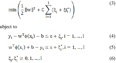
(3)

subject to

D. Min-max Normalization

Min-Max normalization or unity-based normalization is the process of taking data measured in its engineering units and fit the data within value between 0.0 and 1.0. The minimum value is 0.0 and the maximum value is 1.0. This transformation allows a simple way to compare values that are measured on different scales or different units. The following equation is used to normalize value:

(7)

where Xi represents each data point i, XMin is the minima among all the data points, XMax denotes the maxima among all the data points, and Xi,0 to 1 is the data point i normalized between 0 and 1.

E. Performance Evaluation

The model’s performance on the test procedure was measured using the following three metrics: root mean squared error (RMSE) [9], mean absolute percentage error (MAPE) and index of agreement (IA) [10]. RMSE measures residual errors between the observed and predicted values. MAPE evaluates in percentage the difference between the observed values and the predicted values. IA is used to calculate the accuracy between observed values and predicted values. If IA is close to 1, that means predicted values is close to the observed values. In equations 8-10 [9], n is the number of data, Pi represents the predicted value, Oi denotes observed value, and is the average of observed values.

(8)

(9)

(10)

III. PROPOSED WORK

In the proposed work, we divide our analysis process into four main parts: the computation of Pearson’s correlation coefficient, data normalization, k-means clustering, and the ground-level ozone prediction.

A. Pearson’s Correlation Coefficient

Pearson’s correlation coefficient measures the strength of linear relationship between two continuous attributes, i.e., the degree to which their relationship approaches a linear function. It is computed using the following formula:

(11)

where X and Y are two continuous attributes, and represent the average of X and Y, Sx and Sy denote the standard deviation of X and Y, respectively, and N is the amount of data.

The correlation coefficient is a number between -1 and 1; the absolute value of which indicates the strength of the relationship, and the sign of which indicates its direction (positive if the values of one attribute tend to increase with increasing values of the other attribute, and negative otherwise).

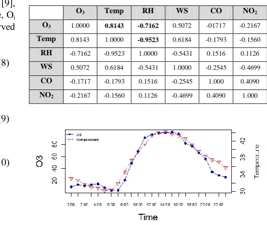
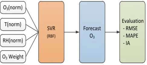
Table II shows the result of Pearson’s correlation coefficient between pollutants (O3, CO, NO2) and meteorological data (temperature -- Temp, relative humidity -- RH, wind speed -- WS). The results show that O3 and temperature have a strong positive relationship between each other, whereas O3 and relative humidity show a strong negative relationship. Meanwhile, temperature and relative humidity also have strong negative relationship. Based upon the Pearson’s correlation analysis, we thus select two independent variables showing the strongest positive and negative relationships, which are temperature and relative humidity, to build the prediction model. Fig. 2 and Fig. 3 also demonstrate these relationships in a graphical form.

TABLEII

Pearson’s correlation coefficient between pollutants and meteorological data.

O3 Temp RH WS CO NO2

O3 1.0000 0.8143 -0.7162 0.5072 -01717 -0.2167 Temp 0.8143 1.0000 -0.9523 0.6184 -0.1793 -0.1560 RH -0.7162 -0.9523 1.0000 -0.5431 0.1516 0.1126 WS 0.5072 0.6184 -0.5431 1.0000 -0.2545 -0.4699 CO -0.1717 -0.1793 0.1516 -0.2545 1.000 0.4090 NO2 -0.2167 -0.1560 0.1126 -0.4699 0.4090 1.000

Fig. 2. Positive relationship between O3 and temperature.

B. K-Means Clustering

K-means clustering is one of the easiest unsupervised learning algorithms widely used to solve the clustering problem. The procedure follows a simple and uncomplicated way to cluster a given data set through a certain number of clusters (supposed k clusters). The main concept is to determine k centers, one of each cluster. These centers should be locating themselves in the excellent way because a different location may cause different result. Therefore, the optimal choice is to locate the k centers as much as possible far away from each other.

The next step is to take each point from a given data set and associate it to the cluster with the nearest center. Data to be clustered are represented as Since the data are p-dimensional, this data set can also be denoted

as The function, , to compute

distance between two data points is normally the Euclidean function. After assigning each and every data point to its closest center, the new k centers have to be recomputed. The assignment of data points to the closest center is iterative until the k centers have not been changed. The final k groups are the grouping of data into k subsets, {C1, …, CK}. In this research, we used three variables as input into k-means clustering. These variables are O3, temperature, and relative humidity because O3 shows high positive correlation to temperature and high negative correlation to the relative humidity, as shown in Fig. 4. Fig. 5 also graphically illustrates three categories of time with different ozone levels based on the clustering result. These 3 categories are low ozone (00:00-07:00), moderate ozone (08:00-09:00 and 21:00-23:00), and high ozone (10:00-20:00).

O3

T

RH

K-Means Clustering

Category 1

Category 2

Category 3

Weight1

Weight2

Weight3

Fig. 4. Temporal-based ozone categorization using k-means clustering.

Category 3

Category 2

Category 1

Fig. 5. Categorized ozone levels using k-means clustering.

After ozone categorization using k-means clustering, the weight has been assign to each category. Low ozone concentration in the early morning, time 00:00-07:00, has weight=1. Moderate ozone concentration, time between 08:00-09:00 and 21:00-23:00, has weight=50. High ozone concentration during the time 10:00-20:00 has weight=100. These categories are shown in Table III.

TABLEIII

Categorizing ozone into three clusters with the different assigned weights.

Ozone Concentration Time Interval Hours Weight

Low 00:00 – 07:00 8 1

Moderate 08:00 – 09:00 and 21:00 – 23:00

5 50

High 10:00 – 20:00 11 100

C. Ground-level Ozone Prediction

Prior to model building, the normalized data were divided into two subsets: training dataset and test dataset. The training dataset is the data in summer months from 2012 to 2015; the test dataset is the data in 2016. SVR with radial basis kernel function and e-intensive loss function has been employed in this work.

O3(norm)

T(norm)

RH(norm)

SVR (RBF)

O3 Weight

Forecast O3

Evaluation - RMSE - MAPE - IA

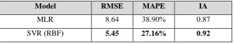
Fig. 6. Ground-level ozone prediction modeling scheme.

IV. EXPERIMENTAL RESULTS

The air pollutant data and meteorological data were collected at northern air quality station in urban area of warm climate from the pollution control department, Chiang Mai, Thailand. In this work, we used data during the summer (February, March, April and May) of 2012, 2013, 2014 and 2015 to predict hourly ground-level ozone concentration in 2016. We focus only these four months because in northern Thailand high ozone concentrations usually occur in the summer. Normalization is our pre-model building step. Table IV illustrates the example for normalized O3, temperature, and relative humidity as a range of 0 to 1.

TABLEIV

Example of normalized O3, Tmp and RH in range [0,1] values.

Max O3 = 135.00 Min O3 = 2.00

Max Tmp = 45.05 Min Tmp = 23.12

Max RH =80.34 Min RH = 3.23

O3 O3

(norm) Tmp

Tmp

(norm) RH

RH (norm)

Fig. 7. Ground-level ozone prediction result from the MLR model (red asterisks), compared against the actual values (black dots).

Fig. 8. Ground-level ozone prediction result from the SVR model (purple plus signs in circle), compared against the actual values (black dots).

Fig. 7 demonstrates the graph showing comparison between ground-level ozone that are obtained from prediction process and ground-level ozone that obtained from observed values. The asterisk signs shows ground-level ozone concentration, which are obtained from the MLR prediction model. The black circles present ground-level ozone concentration, which are obtained from the observed values. Table V shows the MLR model accuracy evaluation, which are measurements from the RMSE, MAPE and IA. The computed errors from the RMSE, MAPE, IA are 8.64, 38.90% and 0.87, respectively.

Fig. 8 represents the comparison between ground-level ozone obtained from the prediction process against the ground-level ozone obtained from the observed values. The plus signs are ground-level ozone concentration obtained from the SVR prediction model and the black circles display ground-level ozone concentration obtained from the observed values. Table V shows the SVR model performance evaluation based on the RMSE, MAPE and IA measurements. The results of RMSE, MAPE, and IA computations are 5.45, 27.16% and 0.92, respectively. For RMSE and MAPE, the lower is the better; but vice versa for IA.

TABLEV

Comparative evaluation between MLR and SVR models.

Model RMSE MAPE IA

MLR 8.64 38.90% 0.87

SVR (RBF) 5.45 27.16% 0.92

V. CONCLUSIONS

In this research, we have proposed the use of support vector regression model for hourly ground-level ozone concentration prediction in the Chiang Mai urban area of Thailand. The SVR model can provide predicting values of ground-level ozone concentration several hours in advance. Pollutants data and meteorological data collected from the pollution control department, Chiang Mai, Thailand during the summer months (February-May) of the years 2012-2015 have been used as training data. The model performance has been tested with the data of the year 2016. The proposed model construction is based on multiple predictors including the hour of the day, the relationship between O3, temperature and relative humidity. The proposed method is to use k-means clustering for categorizing data into three groups with different weighting assignments in each group. Experimental results as comparisons of the prediction accuracy between SVR and MLR models show that SVR model has a greater improve performance in hourly ground-level ozone concentration prediction than the MLR model. Future study shall focus on other important variables contributing to O3 formation. Besides including these variables in the model, we may also use data from the neighbor stations to improve the performance of prediction.

REFERENCES

[1] Y. Zhang, and Y. Wang, “Climate-driven ground-level ozone extreme in the fall over the Southeast United States,” Environmental Sciences, vol. 113, no. 36, pp. 10025 – 10030, Aug. 2016.

[2] T. A. Solaiman, P. Coulibaly, and P. Kanaroglou, “Ground-level ozone forecasting using data-driven methods,” Air Quality, Atmosphere & Health, vol. 1, no. 4, pp. 179 – 193, Dec. 2008. [3] M. A. Barrero, J. O. Grimalt, and L. Canton, “Prediction of daily

ozone concentration maxima in the urban atmosphere,” Chemometrics and Intelligent Laboratory Systems, vol. 80, no. 1, pp. 67-76, Jan. 2006.

[4] C. H. Cheng, S. F. Huang, and H. J. Teoh, “Predicting daily ozone concentration maxima using fuzzy time series based on a two-stage linguistic partition method,” Computer and Mathematics with Applications, vol. 62, no. 4, pp. 2016 – 2028, Aug. 2011.

[5] Y. Feng, W. Zhang, D. Sun, and L. Zhang, “Ozone concentration forecast method based on genetic algorithm optimized back propagation neural networks and support vector machine data classification,” Atmospheric Environment, vol. 45, no. 11, pp. 1979-1985, Apr. 2011.

[6] W. Lu, and D. Wang, “Ground-level ozone prediction by support vector machine approach with a cost sensitive classification scheme,” Science of the Total Environment, vol. 395, no. 2-3, pp. 109-116, Jun. 2008.

[7] V. Gvozdic, E. Kovac-Andric, and J. Brana, “Influence of meteorological factors NO2, SO2, CO and PM10 on the concentration of O3 in the urban atmosphere of eastern Croatia,” Environmental Modelling & Assessment, vol. 16, no. 5, pp. 491-501, Mar. 2011. [8] A. J. Smola, and B. Scholkopf, “A tutorial on support vector

regression,” Statistics and Computing, vol. 14, no. 3, pp. 199-222, Aug. 2004.

[9] A. Z. UI-Saufie, A. S. Yahaya, N. A. Ramli, N. R. Rosaida, and H. A. Hamid, “Future daily PM10 concentrations prediction by combining regression models and feedforward backpropagation models with principle component analysis (PCA),” Atmospheric Environment, vol. 77, no. 1, pp. 621-630, Oct. 2013.

Kedkarn Chaiyakhan is currently a faculty member of the Computer Engineering Department, Raja-mangala University of Technology Isan, Thailand. She received her bachelor degree in Computer Engineering from Rajamangala University of Technology Thanya-buri, Thailand, in 1998, master degree in Computer Engineering from King Mongkut’s University of Technology Thonburi, Thailand, in 2007, and doctoral degree in Computer Engineering from Suranaree University of Technology, Thailand, in 2016. Her current research includes data mining, machine learning, image classification and image clustering.

Pasapitch Chujai is a lecturer at the Electrical Technology Education Department, Faculty of Industrial Education and Technology, King Mongkut’s University of Technology Thonburi, Thailand. She received her bachelor degree in Computer Science from Ramkhamhaeng University, Thailand, in 2000, master degree in Computer and Information Technology from King Mongkut’s University of Technology Thonburi, Thailand, in 2004 and doctoral degree in Computer Engineering, Suranaree University of Technology, Thailand, in 2015. Her current research includes Ontology, Recommendation System, Time Series, and Imbalanced data classification.

Nittaya Kerdprasop is an associate professor at the School of Computer Engineering, Suranaree University of Technology, Thailand. She received her bachelor degree in Radiation Techniques from Mahidol University, Thailand, in 1985, master degree in Computer Science from the Prince of Songkla University, Thailand, in 1991, and doctoral degree in Computer Science from Nova Southeastern University, U.S.A, in 1999. Her research of interest includes knowledge discovery in databases, artificial intelligence, logic and intelligent databases.