Data-Driven Reversible Jump for QTL Mapping

| COMMUNICATIONS

Data-Driven Reversible Jump for QTL Mapping

Daiane Aparecida Zuanetti1_{and Luis Aparecido Milan}

Departamento de Estatística, Universidade Federal de São Carlos, São Carlos, SP, 13565905, Brazil

ABSTRACTWe propose a birth–death–merge data-driven reversible jump (DDRJ) for multiple-QTL mapping where the phenotypic trait is

modeled as a linear function of the additive and dominance effects of the unknown QTL genotypes. We compare the performance of the proposed methodology, usual reversible jump (RJ) and multiple-interval mapping (MIM), using simulated and real data sets. Compared with RJ, DDRJ shows a better performance to estimate the number of QTLs and their locations on the genome mainly when the QTLs effect is moderate, basically as a result of better mixing for transdimensional moves. The inclusion of a merge step of consecutive QTLs in DDRJ is efficient, under tested conditions, to avoid the split of true QTL’s effects between false QTLs and, consequently, selection of the wrong model. DDRJ is also more precise to estimate the QTLs location than MIM in which the number of QTLs need to be specified in advance. As DDRJ is more efficient to identify and characterize QTLs with smaller effect, this method also appears to be useful and brings contributions to identifying single-nucleotide polymorphisms (SNPs) that usually have a small effect on phenotype.

KEYWORDSQTL mapping; model selection; data-driven reversible jump; birth–death–merge movements; mixing of MCMC

G

locating regions associated with quantitative traits in a chromosome. These chromosomal regions are known as quantitative traitloci(QTL) and their location and effects on the phenotypic traits are estimated by genetic markers. The most popular genetic markers are simple sequence repeats (SSR) and single-nucleotide polymorphism (SNP); their location is specified by the linkage map and their genotype is known.

A phenotype is usually modeled as a linear function of the additive and dominance effects of the QTL genotypes and several methods have been developed for the localization and characterization of QTLs. The standard estimation method in experimental crosses is the interval mapping (IM) presented by Lander and Botstein (1989) and Haley and Knott (1992). Lander and Botstein (1989) propose using the EM algorithm (Dempster et al.1977), assuming a single putative QTL at each location on the genome and comparing the hypothesis of a single QTL to the null hypothesis of no segregation QTLs by the logarithm of the odds ratio (LOD score). However, the estimate of the QTL effects can be influenced by the effect of other possible QTLs in adjacent regions since this effect is not

controlled in the model and nonexisting or ghost QTLs can be identified. A ghost QTL appears when two or more QTLs are linked in coupling (meaning that their effects have the same sign) and interval mapping gives a maximum LOD score at a location between the two QTLs (Broman and Speed 1999). Jansen (1993), Jansen and Stam (1994), and Zeng (1994) propose composite-interval mapping (CIM) to control the effect of QTLs located in adjacent regions and avoid the iden-tification of ghost QTLs. They propose to include in the single putative QTL regression model a subset of markers as cofac-tors. Kao et al. (1999) propose multiple-interval mapping (MIM), which considers the effect of all possible QTLs and the epistatic effect between them in a single model. This model, with afixed number of QTLs, is estimated by the EM algorithm and the number of QTLs is selected by model selec-tion methods such as the Akaike informaselec-tion criterion (AIC) and the Bayesian information criterion (BIC), among others.

Bayesian methods for QTL mapping are interesting tools since they allow us to select and estimate the model jointly. Earlier Bayesian approaches were proposed by Stephens and Smith (1993) and Satagopanet al.(1996). The authors esti-mate the locations and effect of a prespecified number of QTLs. In practice, however, the number of QTLs is unknown and must be estimated. Satagopan and Yandell (1996) and Stephens and Fisch (1998) propose variants of reversible-jump (RJ) Markov chain Monte Carlo to estimate it and the remaining parameters of the model jointly. An important characteristic in the chain generated in MCMC is that it mixes Copyright © 2016 by the Genetics Society of America

doi: 10.1534/genetics.115.180802

Manuscript received July 16, 2015; accepted for publication October 30, 2015; published Early Online November 4, 2015.

Supporting information is available online at www.genetics.org/lookup/suppl/ doi:10.1534/genetics.115.180802/-/DC1.

1_{Departamento de Estatística, Universidade Federal de São Carlos, Rodovia Washington}

well;i.e., it moves around the parameter space rather easily and quicklyfinds its stationary distribution. Forming a good Markov chain and monitoring its behavior is delicate and sophisticated work (Broman and Speed 1999).

Over the past decade, different ways to generate proposal parameters in MCMC have been suggested to facilitate the moves between models and accelerate the convergence of the original RJ algorithm. Green and Mira (2001) propose an algorithm that, on rejection, makes a second attempt to move. Regarding the inclusion of a new QTL, Yi and Xu (2002) suggest generating its effects (additive and domi-nance) from the conditionala posterioridistribution. Yiet al. (2005) propose updating the location of a specific QTL and its genotypes together. As a QTL’s location and genotype are correlated, the acceptance probability of a new QTL’s location is higher if its genotype is updated jointly.

To accelerate the search procedure of the correct number of QTLs,K, more suitable and efficient dimensional change can-didates must be generated. For this purpose, we propose a birth–death–merge data-driven reversible jump (DDRJ) for multiple-QTL mapping. It simulates a more likely location for a new QTL using the available data, chooses a QTL to be excluded according to its importance in the current model, or merges the effects of two consecutive QTLs if their genotypes are correlated. Consequently, candidates are more likely to be accepted and the space of possible models is more easily ex-plored. Jain and Neal (2004, 2007) and Saraiva and Milan (2012) show that data-driven methods are effective in simpli-fying the methodology and improving the chain mixing.

The merge movement of consecutive QTLs is efficient un-der tested conditions to avoid identification of false QTLs. Usually, as both QTLs have similar estimated genotypes, the effects of the true QTL are split between the two QTLs and bias the estimate of the number of QTLs and their effects. Split QTLs can be seen as the opposite problem to that of ghost QTLs. The proposed method has also the advantage of providing interval estimates that can be used to analyze the uncertainty of estimates. The usual methods generally provide only point estimates or asymptotic confidence intervals for big samples. This article is organized as follows:Model for Quantitative Traits presents such a model and discusses the likelihood function;Bayesian Approachaddresses the Bayesian approach for the model, including the DDRJ procedure to estimate the number of QTLs; Applications analyzes the performance of DDRJ and compares it with RJ and MIM performance in sim-ulated and real data sets. Finally,Discussionprovides a discus-sion of the methods.

Model for Quantitative Traits

LetY¼ ðY1;Y2;. . .;YnÞbe a quantitative trait ofnindividuals

from an F2 population. Assume this phenotype has been

affected by K QTLs located at positions l¼ ðl1;. . .;lKÞ;

lk,lkþ1 for k¼1;. . .;K21; between m different geno-typed markers with a known linkage map.

PhenotypeYifor theith individual can be modeled by

Yi¼mþX

K

k¼1

akQikþ

XK

k¼1

dkð12jQikjÞ þei; (1)

wherem is the average of expected values of genotypesAA and aa; ak is the additive effect of the kth QTL; dk is the dominance effect of thekth QTL;Qikrepresents the genotype of thekth QTL of theith individual coded as21;0 or 1 foraa; Aa;orAA;respectively,k¼1;. . .;Kandi¼1;2;. . .;n;ei Normalð0;s2Þis the random error; andeiandei9are supposed to be independent fori6¼i9:

The phenotype can also be affected by environmental covariates and interactions among QTLs or between covari-ates and QTLs. The model defined by Equation 1 does not consider these effects, but extensions (modeling environmental covariates asfixed effects, for example) are straightforward.

The data set consists ofy¼ ðy1;y2;. . .;ynÞ;the observations regarding the quantitative trait of nindividuals;Mðn3mÞ;the

markers’genotype are coded as21;0 or 1 foraa;Aa;orAA; respectively; andD¼ fD1;D2;. . .;Dmg;the distances (in cen-timorgans) between each marker and the first marker, where D1¼0:

We assume there is at most one QTL between two consec-utive markers, therefore K,m; and the QTL’s genotype is explained only by flanking markers; i.e., QikjMirk;Milk and

Qik9jMirk9;Milk9are independent for k6¼k9; where Mirk is the

genotype of the marker to the right of thekth QTL for the ith individual andMilkis the genotype of the marker to the left

of thekth QTL for theith individual.

The joint probability distribution of Y and Q; where

Q¼ fQikgis the matrix of theKQTLs genotypes for then individuals, is

f_Y;QjM;Dðy;qÞ ¼Y n

i¼1

fYijqiðyiÞPrðQi¼qijMi;DÞ; (2)

where PrðQi1¼qi1;. . .;QiK¼qiKjMi;DÞ ¼

QK

k¼1PrðQik¼ qikjMirk;Milk;DÞ; for i¼1;. . .;n;

P

qikPrðQik¼qikj Mirk;Milk; DÞ ¼1;forqik¼ 21;0;1;andfis the conditional normal den-sity forYi:

In practice, the number of QTLs K is unknown and the

parameters of the model are u¼ ðK;l;m;a¼ ða1;. . .;aKÞ;

d¼ ðd1;. . .;dKÞ;s2Þ: The likelihood function of u given

Y¼yandQ¼qis

Lðujy;qÞ ¼2ps22n=2exp 2 1 2s2

Xn

i¼1

e2i

( )

3Y

n

i¼1

YK

k¼1

PrQik¼qikjMirk;Milk;D

; (3)

whereei¼yi2m2

PK

k¼1akqik2

PK

k¼1dkð12jqikjÞis the re-sidual of theith observation and PrðQik¼qikjMirk;Milk;DÞis

the conditional probability of the QTL genotype given the

fractions between thekth QTL and itsflanking markers cal-culated by the Haldane distance function. Note that Qik; i¼1;. . .;nandk¼1;. . .;K;is nonobservable and must be estimated.

Without losing the generality and for simplicity, consider the models with one and two QTLs defined, respectively, as

Yi¼mþa1Qi1þd1ð12jQi1jÞ þeiðM1Þ and

Yi¼mþa91Q9i1þa92Q9i2þd19

12Q9i1þd92

12Q9i2

þeiðM2Þ;

fori¼1;. . .;n:Observe ifQ9i1¼Q9i2¼Qi1for all or almost all individuals, a91þa92¼a1 and d91þd92¼d1; the models M1 and M2 are equally or almost equally likely and it can be hard to select the correct model in this situation. The genotype of two loci has a high probability of being equal when they are close on the same chromosome and the model is wrongly estimated if the effect of two or more true close QTLs are merged in only one QTL or if the effect of one true QTL is split with one or more false close QTLs. We note in our simulated data sets, some of them shown inApplications, using multiple QTLs methods to estimate the model, that often methods split the effect of one true QTL with one or more false QTLs. Conventional methodologies for QTL mapping often do not deal well with this problem.

Data availability

File S1contains the conditionala posterioridistributions of parameters. File S2contains DDRJ and RJ effective sample size of the parameters of the models. R codes of DDRJ methos are provided inFile S3andFile S4.

Bayesian Approach

The usual Bayesian methodology for models with unknown Kis the RJ proposed by Green (1995). This method consists of running Metropolis–Hastings steps that either accept or reject different moves, like“birth”or“death”of a QTL. These steps enable transitions from the current model to models of higher or lower dimensions.

ParametersljK;ajK;djK;m,s2_{;and elements ofaandd} are supposed to be independent and the jointa prioridensity foruis written as

pðuÞ ¼pðKÞpðljKÞ Y K

k¼1

pðakÞpðdkÞ

!

pðmÞps2: (4)

Particularly, we consider

1. KUniformð0;1;. . .;m21Þ:

2. akNormalðna;s2aÞ;k¼1;. . .;K;wherena ands2a.0 are known hyperparameters.

3. dkNormalðnd;s2dÞ;k¼1;. . .;K;where nd ands2d.0 are known hyperparameters.

4. m Normalðnm;s2mÞ; where nm and s2m.0 are known hyperparameters.

5. s2_{Inverse-gammaðh}

a;hbÞ;whereha.0 andhb.0 are known hyperparameters.

6. pðljKÞ ¼pðl1;. . .;lKjKÞ ¼pðl1jKÞpðl2jl1;KÞ. . .pðlKj

lK21;KÞ:If there is noa prioriinformation about the QTL’s location, each location is assumed uniformly distributed over the possible loci.

Combining the likelihood function in Equation 3 with the a prioridistributions, we obtain the conditionala posteriori distributions ofmjðy;q;u2mÞ;s2ðy;q;u2s2Þ;a_kjðy;q;u_2akÞ;

dkjðy;q;u2dkÞ;andlkjðy;q;u2lkÞ;k¼1;. . .;K; provided in

Supporting Information,File S1.

The nonobservable genotype Qik; i¼1;. . .;n and k¼1;. . .;K; is simulated and updated by its conditional a posterioridistribution given by

Pr

Qik¼qikjy;q₂qik;M;D

}

Pr

Qik¼qik;Yi¼yijq₂qik;Mirk;Milk;D

¼fYijqiðyiÞPr

Qik¼qikjMirk;Milk;D

; (5)

for qik2 f21;0;1g and where fYijqiðyiÞ is the Normalðmþ PK

k¼1akqikþ

PK

k¼1dkð12jqikjÞ;s2Þdensity function.

From Equation 5,Qikjðy;q₂qik;M;DÞ Multinomialð1;ðpik21;

pik0;pik1ÞÞ;where

pikj¼

fYijqiðyiÞPr

Qik¼jjMirk;Milk;D P

jfYijqiðyiÞPr

Qik¼jjMirk;Milk;D ;

j¼ 21;0;1:

Parametersm,s2;ak;anddkand nonobservable variablesQik; i¼1;. . .;nandk¼1;. . .;K;are updated by Gibbs sampling steps andlkis updated jointly withQkby Metropolis–Hastings steps, in whichlk9is sampled from a UniformðDlk;DrkÞ

distribu-tion and the blockðlk9;Q9kÞis accepted according to probability

Cððlk9;q9kÞðlk;qkÞÞ ¼minð1;AÞ;where

A¼exp

212s2Pni¼1e9i2 exp2ð1=2s2_ÞPn

i¼1e2i

Qn i¼1Pr

Qik¼q9ikMirk;Milk;D Qn

i¼1Pr

Qik¼qikjMirk;Milk;D

3 Qn

i¼1PrðQik¼qikjy;q2qik;M;DÞ Qn

i¼1PrðQik ¼qik9jy;q2qik;M;DÞ

; (6)

ei¼yi2m2

PK

k¼1akqik2

PK

k¼1dkð12jqikjÞ is the residual of theith individual,i¼1;. . .;n;andei9is calculated using q_2q

kandq9k:

DDRJ

The movements that changeKare called birthðbÞ;deathðdÞ;

or merge ðmgÞ moves when a new QTL is included in the

Metropolis–Hastings steps and either increase or reduce the number of QTLs by one at each step.

Considerx¼ ðq;uÞthe current state of the MCMC proce-dure withKQTLs andx9¼ ðq9;u9Þthe proposed movement, where9means a birthðbÞ;a deathðdÞ;or a mergeðmgÞof QTLs. Therefore,K9¼Kþ1 if a birth movement is proposed orK9¼K21 if a death or a merge movement is proposed. This move is accepted according to Metropolis–Hastings probabilityCðx9xÞ ¼minð1;A9Þ;where

A9¼L

u9y;q9

Lðujy;qÞ

pu9

pðuÞ qxjx9

qðx9jxÞ; (7)

andqðjÞis the transition function, described below. At each step, we choose a movement to increase or reduce the number of QTLs as follows:

1. If 0,K,m21;a birth or a death is randomly chosen, according to its probability. Here, we assume PrðbjKÞ ¼1=2 and PrðdjKÞ ¼1=2:

2. IfK¼0;a birth is chosen;i.e., PrðbjKÞ ¼1: 3. IfK¼m21;a death is chosen;i.e., PrðdjKÞ ¼1:

Birth proposal:When a birth movement is chosen, a location is selected for the new QTL in a marker interval that has no QTL and its genotype and effect parameters must be

de-fined. The selection of a location through a Uniform distri-bution can be inefficient, mainly if we have a large number of marker intervals.

If there is a strong association between a marker and a trait, it is reasonable to suppose there is a QTL nearby that marker. Therefore, the association between markers and trait can be used to guide the search for new QTLs in the estimation process. As each marker can be seen as a factor with three levels affecting differently the phenotype mean or the residual mean of the current model, we use the Kruskal–Wallis test statistic to measure this association. TheFstatistics in a one-way analysis of variance could also be used. Higher values indicate

the residual mean is different for the distinct levels of the marker and there is a higher chance of a QTL close to it whose effect is not considered in the current model. Values close to zero indicate the residual mean is the same for all levels of the marker and its contribution to explain the quantitative trait is not relevant or its effect is already considered in the model.

The complete birth step is built as follows:

1. Select a marker to allocate the new QTL from a Multi-nomialð1;ðpb1;. . .;pbmÞÞ; where pbj¼KWj=

Pm j¼1KWj; j¼1;. . .;m;and KWjis the statistics of the Kruskal–Wallis test from residuals of the current model and thejth marker genotype, defined as

KWj¼ ðn21Þ

P3

l¼1nlðrl2rÞ2

P3 l¼1

Pnl

i¼1rli2rÞ2 ;

where nl is the number of individuals in the lth group and the three groups are specified by the genotype of the jth marker,rli is the rank (among all individuals) of the ith individual from the lth group, rl¼

Pnl

i¼1rli=nl; and r¼0:5ðnþ1Þ is the average of all the rli: Note that markers which most affect the residual mean are more likely to be chosen;

2. Assume the j*th marker has been chosen, j*6¼1 and

j*6¼m; and suppose there is no QTL between the

ðj*21Þ and ðj*þ1Þth markers. The new QTL can be located in ½Dj*21;Dj*þ1 and lKþ1 is defined as Dj*21þ

ðDj*þ12Dj*21Þ*Z; where Z Betaða;1Þ and a is calcu-lated according to

E½Z ¼

P​ ðj*_þ1Þ

j¼ðj*_21ÞððDj2Dj*21Þ=ðDj*þ12Dj*þ1ÞÞKWj

P​ ðj*_þ1Þ

j¼ðj*_21ÞKWj

;

i:e:; a¼ E½Z 12E½Z:

Consequently, the expected value oflKþ1is the average of thej*th marker and itsflanking markers’position weighted

by their effect on the residual mean of the current model and the new QTL is more likely to be close to the marker that has the most relevant effect on the residual mean. Note the Betaða;1Þ distribution is Uniformð0;1Þ whenMj*21; Mj*;andMj*þ1 have the same effect on the residual mean and thej*th marker is in the center of½Dj*21;Dj*þ1: If j*¼1;j*¼m;½Dj*21;Dj*or ½Dj*;Dj*þ1 already con-tains a QTL then the new QTL will be located in½D1;D2;

½Dm21;Dm;½Dj*;Dj*þ1;or½Dj*21;Dj*;respectively, and its position is simulated as in step 2, considering only two markers and not three.

3. Sample the genotype of the new QTL for all individuals,

qKþ1;from

PrQiKþ1¼qiKþ1MirKþ1;MilKþ1;D

:

4. SampleaKþ1from its conditionala posterioridistribution consideringqb_{¼ ðq;q}

Kþ1ÞanddKþ1¼0:

5. SampledKþ1from its conditionala posterioridistribution consideringqb_andab_{¼ ða;a}

Kþ1Þ:

6. Sample mb _{from its conditional a posterioridistribution,} consideringqb_;ab_;anddb_{¼ ðd;}

dKþ1Þ: 7. Samples2b

from its conditionala posterioridistribution, consideringqb_;ab_;db_;

andmb_:

Therefore, we have a new set of QTL genotypes and param-etersxb_{¼ ðq}b_;

ubÞ:This transition proposal is denoted byxb_x and its probability is

qxbx¼PrðbjKÞpbj*fZðzÞ

3Y

n

i¼1

PrQiKþ1¼qiKþ1MirKþ1;MilKþ1;D

3 pðaKþ1jy;qb;u2K;Kþ1;lKþ1;dKþ1Þ

3pðdKþ1jy;qb;u2K;Kþ1;lKþ1;aKþ1Þ

3 p

mby;qb;ub_2ðmb_;s2b_Þ;s2

p

s2by;qb;ub_2s2b

;

(8)

where pðjÞ is the conditionala posteriori distribution for each parameter used to sample the candidate values. The accep-tance probability for the birth move is Cðxb_{xÞ ¼minð1;A}b_Þ; whereAb_{is given by Equation 7. The probability of the transition} proposal denoted byxjxb_is

q

xjxb

¼PrðdjKþ1ÞpdKþ1p

mjy;q;u2ðm;s2_Þ;s2 b

3ps2y;q;u2s2

: (9)

Death proposal: Since a death move has been selected, we

choose a QTL from the current model to be deleted. AsQik assumes only values21;0, and 1 andð12jQikjÞ assumes only 0 and 1, fori¼1;. . .;nandk¼1;. . .;K;the current absolute value ofakanddkshows the importance and significance of thekth QTL,i.e., higher absolute val-ues of ak ordkindicate thekth QTL is more relevant to explain the phenotype. The current values of these parameters are useful for the choice of the QTL to be

excluded without changing significantly the predictive

power of the model.

Instead of selecting a QTL to be excluded from a Uniform

ð1;. . .;KÞ;we select it from a Multinomialð1;ðpd1;. . .;pdkÞÞ; where pdk¼ ð1=ðjakj þ jdkjÞÞ=

PK

k¼1ð1=ðjakj þ jdkjÞÞ; for k¼1;. . .;K;i.e., QTLs that exert the strongest effects and are the most relevant to the model are less likely to be se-lected and deleted. Therefore, the acceptance probability of the death movement is improved.

The complete death step is as follows:

1. Select the QTL to be excluded from Multinomial

ð1;ðpd1;. . .;pdKÞÞ;thek*th QTL. 2. Deleteq*

k;l*k;a*k;andd*kfromq;l;a;andd;respectively. 3. Sample md _{from its conditional a posterioridistribution,}

considering onlyK21 QTLs.

4. Samples2dfrom its conditionala posterioridistribution, considering the reduced model.

We have a new set of QTL’s genotypes and parameters xd_{¼ ðq}d_;ud_{¼ ð}

K21;ld;ad_;dd_;

md_;s2d

ÞÞ:This transition pro-posal is denoted byxd_{xand its probability is}

q

xdx

¼PrðdjKÞpdk*p

mdy;qd;ud_2ðmd_;s2dÞ;s2

3p

s2dy;qd;ud_2s2d

; (10)

wherepðjÞis the conditionala posterioridistribution of each parameter used to generate the candidate values.

The acceptance probability for the death movement is Cðxd_{xÞ ¼minð1;A}d_Þ;whereAd_¼1=Ab _{with some suitable} substitutions. The probability of transition proposal denoted byxjxd_{is defined as}

qxjxd¼PrðbjK21Þ

pblk*fZ

lk*2Dlk*21

Dlk*þ12Dlk*21

þpbrk*fZ

lk*2Drk*21

Drk*þ12Drk*21

3 Qn i¼1

PrðQik*¼qik*jMirk*;Milk*;D;lk*Þ

3 p

ak*jy;q;ud_2ðK21Þ;K;lk*;dk*

3p

dk*jy;q;ud_2ðK21Þ;K;lk*;ak*

3 p

mjy;q;u_2ðm;s2_Þ;s2 d

ps2y;q;u2s2

; (11)

wherelk*is the marker on the left of thek*  th QTL andrk*is the marker on the right of thek* th QTL.

Note that if we first choose a birth movement in state x, giving xb_{;and then choose the death of the ðKþ1Þth} QTL, we can recoverxand statexis likely to be recovered after a birth process of xd_{:If the candidate movement is} not accepted, the chain remains in the current model, the value ofKdoes not change, and the remaining parameters

of the model are updated by Metropolis–Hastings or Gibbs steps.

Merge proposal:Instead of proposing data driven with only birth and death steps, we also include a merge movement in the procedure since the model can be wrongly estimated if the effect of a true QTL is split between two or more false QTLs. The split of a QTL may happen if a QTL appears very close to an existent QTL and, as their genotypes are very similar, both are in the model and split the additive and dominance effect that would be of only one QTL. The death of one of these QTLs is not generally accepted since the effects of both QTLs are relevant to explain the phenotype variability. The merge moves of two consecutive QTLs are usually accepted and effective to avoid split QTLs since the effect of the QTL that is removed from the model is added to the effect of an adjacent QTL and the predictive power of the model does not change significantly.

For merging two QTLs we must choose a pair of consec-utive QTLs to be merged and choose one QTL to be removed from the model. Its effects are added to the effect of the other QTL. We propose to build a data-driven merge can-didate as follows:

1. Select a pair of consecutive QTLs to be merged from Multinomialð1;ðpmg12;pmg23;. . .;pmg_ðK21ÞKÞÞ; where pmgkj¼ Vkj=

PK21

k¼1

PK

j¼kþ1Vkj; k¼1;. . .;K21 and j¼ kþ1;. . .;K;andVkj is Cramér’sVmeasure of associa-tion between the genotypes of thekth and thejth QTLs. Note that pairs of successive QTLs with more associated genotypes have higher probability to be merged since the split happens between QTLs with similar genotype.

Suppose the pair of QTLs k* and k*þ1 has been

selected.

2. Choose the k*th or ðk*þ1Þth to be excluded from

the current model, according to pdk¼ ð1=ðjakj þ jdkjÞÞ=

Pk*þ1

k¼k*ð1=ðjakj þ jdkjÞÞ;k¼k*;k*þ1:Consider that the

ðk*þ1Þth has been chosen to be excluded.

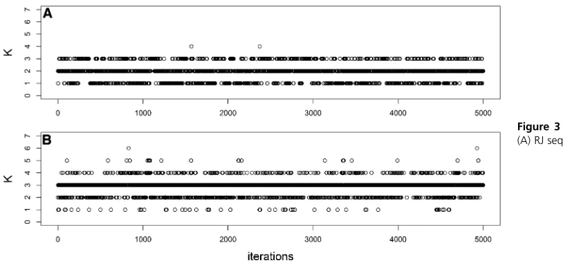
Figure 3Trace plot ofK fors¼1:5:

3. Deleteqk*þ1;lk*þ1;ak*þ1;anddk*þ1fromq;l;a;andd; respectively.

4. Updateak*;dk*;m, ands2;successively, from their condi-tionala posterioridistribution consideringqmg_;amg_;and dmgwithk21 QTLs.

Instead of adding the value ofak*þ1anddk*þ1toak*and

dk*;respectively, we propose to updateak*anddk*from their conditionala posterioriprobability, using the reduced model. It is equivalent since we remove the effects of theðk*þ1Þth QTL from the current model to updateak*anddk*and sim-plify the calculation of merge acceptance probability since is not necessary to define deterministic transformations to re-duce the dimension of the model.

We have a new set of QTL’s genotypes and parameters

xmg_{¼ ðq}mg_;umg_{¼ ð}

K21;lmg;amg_;dmg_;

mmg_;s2mg

ÞÞ:This tran-sition proposal is denoted byxmg_{jxand its probability is}

qðxmgjxÞ ¼pmgk*ðk*þ1Þpdk*þ1

3p

ak*jy;qmg;K21;lmg;amg_2ak_*;d

mg_;

m;s2

3p

dk*jy;qmg;K21;lmg;amg;dmg_2dk

*;m;s

2

3p

mmgjy;qmg;u_2ðmg_mmg_;s2mg_Þ;s

2

3ps2mgy;qmg;umg_2s2mg

; (12)

wherepðjÞis the conditionala posterioridistribution of each parameter used to sample the candidate values.

The acceptance probability for the merge movement isCðxmg_{jxÞ ¼minð1;A}mg_Þ;whereAmg_{is defined by Equation} 7. The probability of a transition proposal denoted byxjxmg that represents a split of thek*th QTL is defined as

qðxjxmgÞ ¼ pblk*þ1fZ

lk*þ12Dlk*þ121

Dlk*þ1þ12Dlk*þ121

þpbrk*þ1fZ

lk*þ12Drk*þ121

Drk*þ1þ12Drk*þ121

!

3Yn

i¼1

PrQ_ik*þ1¼q_ik*þ1Mirk*þ1;Milk*þ1;D;lk*þ1

3 p

ak*þ1jy;q;umg₂ðK21Þ;K;lk*þ1;dk*þ1¼0

3p

dk*þ1jy;q;umg₂ðK21Þ;K;lk*þ1;ak*þ1

3 pðak*jy;q;u2ak*Þpðdk*jy;q;u2dk*Þ

3 pmjy;q;u2ðm;s2_Þ;s2 mg

ps2y;q;u2s2

; (13)

where lk*þ1 is the marker on the left of the ðk*þ1Þ th QTL andrk*þ1is the marker on the right of theðk*þ1Þ th QTL.

Since we include the QTL merge move only to avoid split QTLs, we do not include a QTL split step in this procedure. However, a split step could be easily included in the algo-rithm, using the transition function of a split movement qðxsp_{jxÞ ¼qðxjx}mg_{Þdefined in Equation 13.}

Algorithm:The birth–death–merge DDRJ is specified as follows:

1. Initialize a configuration foruandq: 2. For thelth iteration,l¼1;. . .;L;

a. Choose a death or birth movement. b. Generate the candidate values ofx9:

c. Accept the proposal with probability Cðx9xÞ;where9 means eitherbord.

i.If a birth movement has been accepted, do KðlÞ_¼ Kðl21Þþ1 and considerxb:

ii.If a death movement has been accepted, do KðlÞ_¼

Kðl21Þ_{21 and considerx}d_:

iii. If no movement has been accepted, doKðlÞ_¼Kðl21Þ

and considerx.

d. If KðlÞ_{$2; generate and evaluate the acceptance of a}

merge of a QTLs pair. If a merge movement has been accepted, doKðlÞ_¼KðlÞ_{21 and considerx}mg_:

e. Updatelk;k¼1;. . .;KðlÞ:

f. UpdateQik;i¼1;. . .;nandk¼1;. . .;KðlÞ;from its con-ditionala posterioridistribution.

g. Updateakanddk;k¼1;. . .;KðlÞ;from their conditional a posterioridistributions.

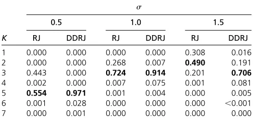
Table 2 A posterioriprobability forK

s

0.5 1.0 1.5

K RJ DDRJ RJ DDRJ RJ DDRJ

1 0.000 0.000 0.000 0.000 0.308 0.016

2 0.000 0.000 0.268 0.007 0.490 0.191

3 0.443 0.000 0.724 0.914 0.201 0.706

4 0.002 0.000 0.007 0.075 0.001 0.081

5 0.554 0.971 0.001 0.004 0.000 0.005

6 0.001 0.028 0.000 0.000 0.000 ,0.001

7 0.000 0.001 0.000 0.000 0.000 0.000

The highest a posteriori probability estimate for each case is in boldface type.

Table 1 ESS ofKsequences

Error variability RJ DDRJ

s¼0:5 3 357

s¼1:0 159 330

h. Updatemfrom its conditionala posterioridistribution. i. Updates2 _{from its conditionala posterioridistribution.}

This algorithm is implemented in R language and the codes are available in File S3 and File S4. R is a free software environment for statistical computing and graphics and more details are found in its homepage, “https://www.r-project. org”.

Applications

We apply the proposed method to simulated and real data sets and compare the performance of the RJ, DDRJ, and MIM methodologies. Although the computational efficiency is an important feature of the methods, we focus on analyzing and comparing their performance in selecting and estimating the correct model. We set hyperparameters na¼nd¼nm¼0;

s2a¼s 2 d¼s

2

m¼100; and ha¼hb¼0:1: This setup pro-vides a priori distributions with large variability and weak information about the parameters.

Simulated data sets

We simulate a high-dimension linkage map with 450 loci that are allocated on a large chromosome of 450 cM (average distance between the loci is 1 cM) and their genotype for an F2 population of 300 individuals by QTL Cartographer 2.5 software available at “http://statgen.ncsu.edu/qtlcart/WQTLCart.htm”

(Basten et al. 1997). We choose K¼5 loci located at

l¼ f15:0;82:4;299:8;363:1;391:1gto be the QTLs and sim-ulate the phenotype using a¼ ð20:60;0:90;0:25;20:40; 0:40Þ; d¼ ð0:30;0:05;20:25; 0:15;20:15Þ; m¼20; and three values of s ð0:5;1:0;1:5Þ:The effects of the first and the second QTLs are stronger and are easily identified, the fourth andfifth QTLs have opposite effects, and the effect of the third QTL is the weakest.

We run RJ and DDRJ chainsL¼55;000 iterations, discard thefirst 5000 iterations, and take one for every 10 iterations. The chains are initialized withK¼0:Convergence is verified using trace plots.

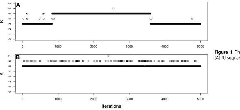
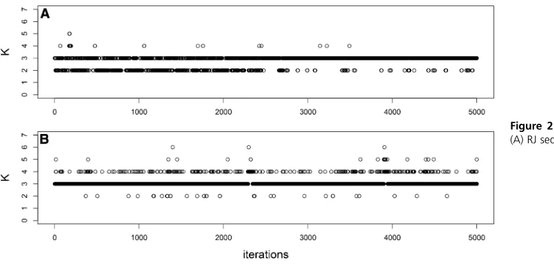
Figure 1, Figure 2, and Figure 3 show the RJ and DDRJ trace plots of Kfor s¼0:5;1.0, and 1.5, respectively. We observe DDRJ chains show better mixing since they easily move around the models space throughout the chain as a con-sequence of better proposal candidates. The RJ chain moves with greater difficulty between the possible models and it can get stuck in a specific model for longer periods even if it is a wrong model. Whens¼0:5;we observe a very poor mix-ing of the RJ chain since it gets stuck for long periods (at the

beginning and end of the chain) in the model with K¼3

(wrong model). When s¼1:0; the RJ chain moves easily around the models space in the beginning of the chain but not in its end.

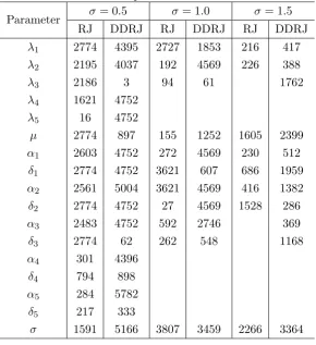
We also analyze the mixing of the chains by their effective sample size (ESS) (Kasset al.1998), which is the number of effectively independent draws from thea posterioridistribution. Table

A large discrepancy between the ESS and the simulation sample size indicates poor mixing. Table 1 shows the ESS

for the RJ and DDRJKsequences and we observe the DDRJ

ESS is larger than the RJ ESS, which confirms a better mixing of DDRJ chains. We observe a very poor mixing of the RJ chain mainly fors¼0:5:DDRJ and RJ ESSs of the remaining parameters of the models are shown in Table A ofFile S2and DDRJ ESSs are in most cases larger than RJ ESSs.

Table 2 showsa posterioriprobabilities forKcalculated as the relative frequency of each value ofKin the sequence. The highesta posterioriprobability estimate for each situation is in boldface type and the argument that maximizes this prob-ability is the estimate of K. In situations where the genetic effects of QTLs are strong compared with the size of the error variability (s¼0:5) both methodologies estimate correctly K¼5:However, as a result of weak mixing, the RJ chain gets stuck inK¼3 for long periods and tends to underestimate the a posteriori probability of K. Since s¼0:5 represents a small variability of the random error and, consequently, the effect of QTLs is more evident, the choice of the correct model should be precise. Whens$1:0;the opposite fourth andfifth QTLs, although they have higher additive effect than the third QTL, are not identified by RJ and DDRJ since their effects cancel each other. Fors¼1:5;the RJ procedure esti-mates onlyK¼2 and shows greater difficulties in locating the QTLs.

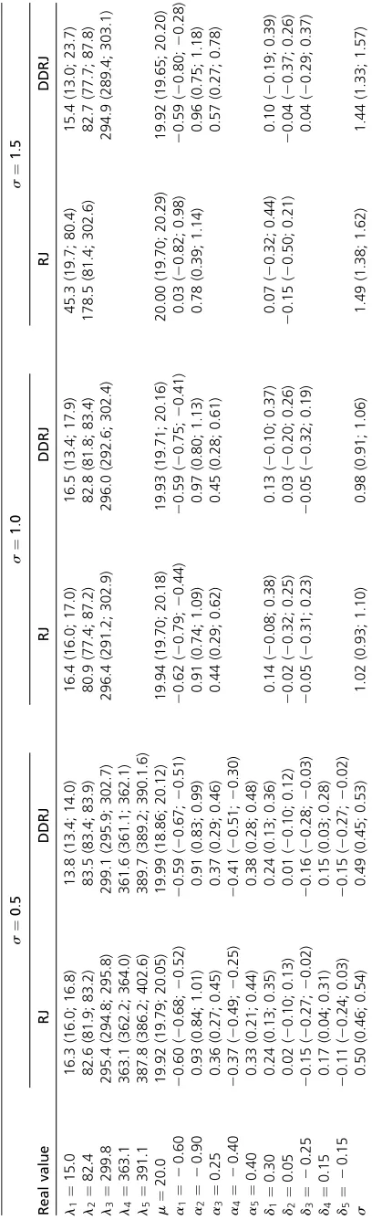
Table 3 shows the estimates (a posteriori average) of

parameters and their 95% credibility interval. The estimates of both methodologies are similar when s¼0:5 and close to the true values. The DDRJ point estimates of the additive and the dominance effect of the fourth and fifth QTLs are closer to the true simulated parameters than the RJ esti-mates. Zero belongs to the RJ credibility interval ofd5:The additive and dominance effects of the third QTL are the worst estimate in both methods. Whens¼1:0;RJ and DDRJ

esti-mates for the model with K¼3 QTLs are similar and the

additive and dominance effects estimates of the third QTL are also the worst estimate in both methods. For s¼1:5; RJ shows a low performance to estimate the number of QTLs and the parameters associated with them. The RJ point mates are different from the parameters and interval esti-mates are large.

We also analyze the simulated data sets, using the MIM method available in QTL Cartographer. The main model selection criterion available in QTL Cartographer to select the number of QTLs is BIC ¼ 22logðLð^uy;qÞÞ þpcðnÞ; whereu^is the maximum-likelihood estimator ofu;pis the number of free parameters to be estimated, andcðnÞ ¼logðnÞ:

Other definitions of cðnÞ are used and available in QTL Cartographer such as cðnÞ ¼2 (AIC), cðnÞ ¼2logðlogðnÞÞ; cðnÞ ¼2logðnÞ;cðnÞ ¼3logðnÞ;andcðnÞ ¼10XlogðnÞ;where we define X¼0:01: We choose the MIM forward search method to estimate the initial model and test the six model selection criteria to optimize QTLs positions, search for new QTLs, and test existing QTLs. We report the results of cðnÞ ¼logðnÞ;which shows the best results for the simulated data sets.

The MIM method combined with BIC model selection methodologies and optimization procedures of QTL location and effect estimatesK¼6;3;3 fors¼0:5;1:0;and 1.5, re-spectively. Table 4 shows the MIM estimates of the remaining parameters of the models. The method identifies one non-existing QTL at 9.0 cM whens¼0:5 and the additive and dominance effects of the second QTL are biased. We observe that if we sum the estimates of additive and dominance effects of first and second QTLs, we have estimates closer to additive and dominance effects of the QTL located at 15.0 cM; that is, the effects of the true QTL estimated at 14 cM are split with a false QTL identified at 9 cM. When

s¼1:0 and 1.5, the opposite fourth andfifth QTLs are not identified and the DDRJ estimates of the remaining parame-ters, especially estimates associated with the third QTL that has weaker effects, are better than MIM estimates. We do not have a confidence interval to analyze the uncertainty of the parameters.

Unlike BIC (cðnÞ ¼logðnÞ), we stop the AIC, BIC-like criteria with cðnÞ ¼2logðlogðnÞÞand cðnÞ ¼0:1logðnÞ esti-mation when they wrongly identify K¼12;9; and 9 sig-nificant QTLs for s¼0:5;1:0; and 1.5 located at ^l ¼

f9:0;14:0;83:4;86:4;91:5;298:8;339:8;351:2;360:2;363:1; 388:2;390:1g; l^ ¼ f10:0;14:0;83:4;293:8;301:8;309:8; 337:8;388:1;390:1g;andl^¼ f3:0;9:0;14:0;83:4;86:4;91:5; 293:8;338:8;410:1;390:1g;respectively. The BIC-like crite-rion with cðnÞ ¼2logðnÞ estimates K¼3 significant QTLs located at l^¼ f14:0;83:4;293:8g for all values of s and the BIC-like criterion with cðnÞ ¼3logðnÞ estimates K¼3 QTLs located at l^¼ f14:0;83:4;296:8gfor s¼0:5;K¼2 QTLs located atl^¼ f15:0;83:4gfors¼1:0;andK¼1 sig-nificant QTL located atl^¼83:5 fors¼1:5:Therefore, we observe the MIM method combined with BIC model selection is sensitive tocðnÞchoice for these simulated data sets; that is, depending on thecðnÞchoice, the method overestimates or underestimates the number of QTLs. If the data were not simulated and we did not know the correct model, we could estimate the model by the six MIM model selection criteria and select the estimated model that was the most frequent

Table 4 MIM estimates of the parameters

Parameter Real value s¼0:5 s¼1:0 s¼1:5

l ð15:0;82:4;299:8;363:1;391:1Þ ð9:0;14:0;83:4;298:8;363:1;390:1Þ ð14:0;83:4;293:8Þ ð14:0;83:4;293:8Þ

a ð20:60;0:90;0:25;20:40;0:40Þ ð0:24;20:80;0:89;0:40;20:43;0:40Þ ð20:58;0:96;0:47Þ ð20:59;0:98;0:61Þ

between all criteria. In this case, we would choose, for all values ofs, the model estimated by the AIC, BIC-like criterion with cðnÞ ¼2logðlogðnÞÞandcðnÞ ¼0:1logðnÞ;which is the worst estimated model.

Real data set

We apply RJ and DDRJ to the bone mineral density data set. It consists of 661 female F2mice derived from matings of F1

individuals from NZB/B1NJ 3 RF/J parents. This cross is

designed to identify the genetic loci regulating femur me-chanical properties, geometric properties, and bone mineral density (BMD). The data have 94 genetic markers located in 19 chromosomes. NZB, RF, and heterozygous markers are coded as 1,21;and 0, respectively. The data were downloaded from the site“http://qtlarchive.org/db/q?pg=projlist”.

Twenty-three phenotypes were measured in all individuals; however, we analyze only the total femur volumetric BMD in milligrams per cubic centimeter. The trait was log-transformed before analysis to be comparable with Wergedalet al.(2006) and Coxet al.(2009) results.

We runL¼110;000 RJ iterations, discard thefirst 10,000 and take one for every 10 iterations. We run L¼55;000 DDRJ iterations, discard thefirst 5000, and take one for every 10 iterations. The sequences are initialized withK¼0 and, in DDRJ, we update the birth candidate 10 times before evalu-ating its acceptance, as proposed by Green and Mira (2001). We analyze the convergence and conclude the number of iterations is sufficient for reliable results.

Table 5 shows the a posterioriDDRJ probability (relative frequency) forKin each chromosome whose value is evidence of a QTL presence. Thea posterioriprobability of the model with one QTL is 0.67 in chromosome 7, 0.42 in chromosome 11, 0.38 in chromosome 19, 0.33 in chromosome 9, and 0.25 in mosome 1, which represents strong evidence of a QTL in

chro-mosome 7 since K¼1 is the argument that maximizes the

a posterioriprobability ofKand moderate probability in chro-mosomes 1, 9, 11, and 19 since, despite that the maximum a posterioriprobability is not forK¼1;it is.0.25. In chromo-somes 10, 12, 17, and 18, the probability of a QTL is not neg-ligible. Depending on the cost and researcher interest, these loci can be studied in more detail. Therefore, we identify at least K¼5 QTLs regulating bone mineral density.

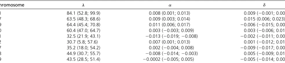
Table 6 shows estimates and 95% credibility intervals for QTLs’locations (centimorgans) and additive and dominance effects in chromosomes 1, 7, 9, 10, 11, 12, 17, 18, and 19. Additive and dominance effects explain how QTLs genotypes are associated to bone mineral density and their estimates are small (close to zero) because of the scale of the log(BMD). Although the chance of a QTL in chromosomes 10, 17, and 19 is not negligible, zero belongs to their additive and domi-nance effects 95% credibility interval. Therefore, DDRJ iden-tifies relevant QTLs at chromosomes 1, 7, 9, 11, 12, and 18. We also analyze these data by a RJ and MIM forward search method combined with BIC model selection (cðnÞ ¼logðnÞ), which shows better results in the simulated data sets. We observe only RJ low a posteriori probabilities 0.0006, 0.0009, and 0.027 for one QTL in chromosomes 7, 9, and 11, respectively. MIM identifies one QTL in chromosomes 1, 7, 9, 11, and 12 located at 88, 65, 70, 34, and 28 cM, re-spectively. The MIM point estimates of additive and domi-nance effects are a^¼ ð0:009;0:009;0:012;20:014;0:009Þ and ^d¼ ð0:008;0:016;20:005;20:004;0:004Þ:The MIM effect estimates are close to DDRJ estimates; however, we do not have information about MIM estimates uncertainty. Wergedalet al.(2006) use a three-stage strategy and LOD score to identifyK¼5 QTLs located in chromosomes 3, 7, 10, 11, and 18 at 10-, 65-, 65-, 40-, and 50-cM positions, respectively.

If we use the DDRJa posterioriprobability ofKas evidence of QTL presence, we observe DDRJ, MIM, and Wergedal methodologies identify QTLs in chromosomes 7 and 11; DDRJ and MIM identify three more QTLs in chromosomes 1, 9, and 12; and DDRJ and Werdegal methods identify an-other QTL in chromosome 18. The Werdegal method also identifies one QTL in chromosomes 3 and 10 whose credibil-ity interval of additive effect and dominance effect contains zero. Therefore, for this data set, DDRJ methodology

identi-fies QTLs with strong and weak effects in BMD that are not identified by other QTL mapping methods.

Discussion

We propose a birth–death–merge DDRJ for QTL mapping in

an F2 population with an unknown number of QTLs. We

compare the performance of the proposed method with

Table 5 DDRJA posterioriDDRJ probability forKin each chromosome

Chromosome

K 1 2 3 4 5 6 7 8 9 10

0 0.60 0.93 0.90 0.86 0.95 0.92 0.30 0.85 0.63 0.76

1 0.25 0.06 0.09 0.11 0.04 0.06 0.67 0.12 0.33 0.17

2 0.13 0.01 0.01 0.03 0.01 0.02 0.03 0.03 0.03 0.06

$3 0.02 0.00 0.00 0.00 0.00 0.00 0.00 0.00 0.01 0.01 Chromosome

K 11 12 13 14 15 16 17 18 19

0 0.47 0.79 0.88 0.91 0.92 0.94 0.76 0.82 0.59

1 0.42 0.18 0.11 0.08 0.07 0.05 0.21 0.16 0.38

2 0.10 0.03 0.01 0.01 0.01 0.01 0.02 0.02 0.03

traditional RJ and MIM combined with a model selection method and optimization procedures that are the most popular methodologies for QTL mapping in experimental crosses. Al-though computational efficiency is an important feature of the methods, we focus on analyzing and comparing their perfor-mance in identifying significant QTL regions.

DDRJ shows a better performance to identify and estimate QTLs mainly when their effects are moderate and RJ does not identify them. The better performance of DDRJ occurs be-cause it facilitates the moves around the models space and improves the chain mixing as a consequence of better pro-posals in transdimensional moves. Unlike DDRJ, the RJ method moves with greater difficulty between the possible models and it can get stuck in a specific model for longer periods even if it is a wrong model. Compared with MIM combined with model selection methods, DDRJ also shows better performance in identifying QTL regions and provides uncertainty information for all parameters through credibility intervals. For simulated data sets, MIM shows sensitivity to the choice of model selection criterion and, depending on the criterion choice, the method overestimates or underestimates the number of QTLs. As QTLs single effects are not so high in practice, mainly the effect of SNP QTLs (Yanget al.(2010)), the proposed methodology appears to be useful and brings contributions to identification and characterization of QTLs. The DDRJa posterioriprobability ofKis evidence of QTL presence and, even when this value is not maximum for K.0;it allows us to specify regions that can be further ex-plored by genetic researchers. The application in a real data set illustrates an example where DDRJ identifies QTLs with strong, moderate, and weak effects on the phenotype that are not identified by RJ, MIM, or other QTL mapping methods.

The inclusion of merge moves in DDRJ is efficient under analyzed data sets to avoid the split of a true QTL effect with one or more false QTLs. The conventional methodologies usually deal with a ghost QTL that appears between two or more QTLs linked in coupling and is generally more significant than the true QTLs. The problem presented here is the opposite of that of a ghost QTL since the true QTLs share their importance with one or more false QTLs. Ghost QTLs are usually avoided by multiple-QTL mapping methods and merge moves included in DDRJ reduce the chance of split QTLs. Since we include the QTLs merge move only to avoid split QTLs, we do not include a QTL split step in this procedure.

The R codes of birth–death–merge data-driven reversible jump are available inFile S3andFile S4and we are improv-ing them to be more efficient and user friendly.

The amplitude of the DDRJ credibility interval of QTLs’ location is large when error variability is higher. To improve the DDRJ performance, we can estimate the genotype of

a QTL using more than the two flanking markers or using

nonconjugate samplers, and analyze the results in future work. The proposed data-driven method can be extended to generalized linear models and identifies QTLs that affect binary or discrete phenotypes or for QTL mapping in pedigree data in which the individuals’genotype is correlated if they are relatives and improves SNP mapping methods that have a smaller single effect on the phenotype.

Acknowledgment

The authors thank two referees for useful comments and suggestions that improved the manuscript.

Literature Cited

Basten, C. J., B. S. Weir, and Z.-B. Zeng, 1997 QTL Cartographer:

A Reference Manual and Tutorial for QTL Mapping. Department of Statistics, North Carolina State University, Raleigh, NC.

Broman, K. W., and T. Speed, 1999 A Review of Methods for

Iden-tifying QTLs in Experimental Crosses(Lecture Notes-Monograph

Series), pp. 114–142. Hayward, California.

Cox, A., C. L. Ackert-Bicknell, B. L. Dumont, Y. Ding, J. T. Bellet al.,

2009 A new standard genetic map for the laboratory mouse.

Genetics 182: 1335–1344.

Dempster, A. P., N. M. Laird, and D. B. Rubin, 1977 Maximum

likelihood from incomplete data via the EM algorithm. J. R. Stat.

Soc. B Methodol. 39: 1–38.

Green, P. J., 1995 Reversible jump Markov chain Monte Carlo

computation and Bayesian model determination. Biometrika

82(4): 711–732.

Green, P. J., and A. Mira, 2001 Delayed rejection in reversible

jump Metropolis–Hastings. Biometrika 88(4): 1035–1053.

Haley, C. S., and S. A. Knott, 1992 A simple regression method for

mapping quantitative trait loci in line crosses using _flanking

markers. Heredity 69(4): 315_–324.

Jain, S., and R. M. Neal, 2004 A split-merge Markov chain Monte

Carlo procedure for the Dirichlet process mixture model. J.

Comput. Graph. Stat. 13: 158–182.

Jain, S., and R. M. Neal, 2007 Splitting and merging components

of a nonconjugate Dirichlet process mixture model. Bayesian

Anal. 2(3): 445–472.

Table 6 DDRJ estimates and95% credibility intervals of parameters

Chromosome l a d

1 84.1 (52.8; 99.9) 0.008 (0.001; 0.013) 0.009 (20.001; 0.002)

7 63.5 (48.3; 68.6) 0.009 (0.003; 0.014) 0.015 (0.006; 0.023)

9 64.4 (45.4; 70.8) 0.011 (0.006; 0.017) 20.006 (20.015; 0.005)

10 60.4 (47.0; 64.7) 0.003 (20.003; 0.009) 0.003 (20.006; 0.010)

11 32.5 (21.9; 43.1) 20.013 (20.019;20.008) 20.002 (20.011; 0.007)

12 30.7 (5.8; 57.6) 0.007 (0.001; 0.013) 0.001 (20.012; 0.015)

17 35.2 (18.0; 54.2) 0.002 (20.004; 0.008) 20.009 (20.017; 0.001)

18 44.9 (30.7; 55.7) 20.008 (20.014;20.003) 0.005 (20.009; 0.015)

Jansen, R. C., 1993 Interval mapping of multiple quantitative trait

loci. Genetics 135: 205–211.

Jansen, R. C., and P. Stam, 1994 High resolution of quantitative

traits into multiple loci via interval mapping. Genetics 136:

1447–1455.

Kao, C.-H., Z.-B. Zeng, and R. D. Teasdale, 1999 Multiple interval

mapping for quantitative trait loci. Genetics 152: 1203–1216.

Kass, R. E., B. P. Carlin, A. Gelman, and R. M. Neal, 1998 Markov

chain Monte Carlo in practice: a roundtable discussion. Am.

Stat. 52(2): 93–100.

Lander, E. S., and D. Botstein, 1989 Mapping Mendelian factors

underlying quantitative traits using RFLP linkage maps.

Genet-ics 121: 185_–199.

Saraiva, E. F., and L. A. Milan, 2012 Clustering gene expression

data using a posterior split-merge-birth procedure. Scand. J.

Stat. 39(3): 399–415.

Satagopan, J. M., and B. S. Yandell, 1996 Estimating the number

of quantitative trait loci via Bayesian model determination.

Pro-ceedings of the Joint Statistical Meetings.

Satagopan, J. M., B. S. Yandell, M. A. Newton, and T. C. Osborn,

1996 A Bayesian approach to detect quantitative trait loci

us-ing Markov chain Monte Carlo. Genetics 144: 805–816.

Stephens, D., and R. Fisch, 1998 Bayesian analysis of quantitative

trait locus data using reversible jump Markov chain Monte

Carlo. Biometrics 54: 1334–1347.

Stephens, D., and A. Smith, 1993 Bayesian inference in

multi-point gene mapping. Ann. Hum. Genet. 57(1): 65–82.

Wergedal, J. E., C. L. Ackert-Bicknell, S.-W. Tsaih, M. H.-C. Sheng,

R. Liet al., 2006 Femur mechanical properties in the F2

prog-eny of an NZB/B1NJ3RF/J cross are regulated predominantly

by genetic loci that regulate bone geometry. J. Bone Miner. Res.

21(8): 1256–1266.

Yang, J., B. Benyamin, B. P. McEvoy, S. Gordon, A. K. Henderset al.,

2010 Common SNPs explain a large proportion of the

herita-bility for human height. Nat. Genet. 42(7): 565_–569.

Yi, N., and S. Xu, 2002 Mapping quantitative trait loci with

epi-static effects. Genet. Res. 79(02): 185–198.

Yi, N., B. S. Yandell, G. A. Churchill, D. B. Allison, E. J. Eisenet al.,

2005 Bayesian model selection for genome-wide epistatic

quantitative trait loci analysis. Genetics 170: 1333–1344.

Zeng, Z.-B., 1994 Precision mapping of quantitative trait loci.

Ge-netics 136: 1457–1468.

GENETICS

Supporting Information

www.genetics.org/lookup/suppl/doi:10.1534/genetics.115.180802/-/DC1

Data-Driven Reversible Jump for QTL Mapping

Daiane Aparecida Zuanetti and Luis Aparecido Milan

1

Conditional

a posteriori

distribution of parameters

Combining the likelihood function with the

a priori

distributions, we obtain the conditional

a posteriori

distribution of

µ

|

(

y,

q,

θ

),

σ

|

(

y,

q,

θ

),

α

|

(

y,

q,

θ

),

δ

|

(

y,

q,

θ

) and

λ

|

(

y,

q,

θ

),

k

= 1

, ..., K

.

Specifically,

µ

|

(

y,

q,

θ

)

∼

Normal





Pn

i=1

(

PK

k=1αkqik−

PK

k=1δk(1−|qik|)

)

σ2 +

νµ σ2µ n

σ2+

1

σ_µ2

,

σ2+

1

σ2_µ





,

σ

|

(

y,

q,

θ

)

∼

Inverse-gamma

n 2

+

η

,

Pn

i=1

(

PK

k=1δk(1−|qik|)

)

2

2

+

η

,

α

|

y,

q,

θ

k∗

∼

Normal





Pn

i=1qik∗

(

P

k6=k∗αkqik−

PK

k=1δk(1−|qik|)

)

σ2 +_σνα2

α

Pn

i=1q2ik∗

σ2 +

1

σ2α

,

i=1q2ik∗

σ2 +

1

σ2α





,

δk∗ |

(

δk∗

)

Normal



     

Pn

i=1(1−|qik∗ |)

(

P

k6=k∗δk(1−|qik|)

)

σ2 +_σνδ2

δ

Pn

i=1(1−|qik∗ |)2

σ2 + 1_σ2

δ

,Pn 1

i=1(1−|qik∗ |)2

σ2 + 1_σ2

δ



     

and

π λ

|

y,

q,

θ

k∗

∝

i=1P r

(

)

Dm−(K−k∗)−D_rk∗−1

, for

k

2

Additional information about RJ and DDRJ chains of high

dimension simulated data sets

Table A shows the effective sample size (ESS) of RJ and DDRJ chains of all parameters of

the estimated models for simulated data sets. We observe DDRJ ESS is higher than RJ ESS in

most cases which confirms a better mixing of DDRJ chains.

Table A: Effective sample size of RJ and DDRJ chains.

Parameter

σ

= 0

.

5

σ

= 1

.

0

σ

= 1

.

5

RJ

DDRJ

RJ

DDRJ

RJ

DDRJ

λ

2774

4395

2727

1853

216

417

λ

2195

4037

192

4569

226

388

λ

2186

3

94

61

1762

λ

1621

4752

λ

16

4752

µ

2774

897

155

1252

1605

2399

α

2603

4752

272

4569

230

512

δ

2774

4752

3621

607

686

1959

α

2561

5004

3621

4569

416

1382

δ

2774

4752

27

4569

1528

286

α

2483

4752

592

2746

369

δ

2774

62

262

548

1168

α

301

4396

δ

794

898

α

284

5782

δ

217

333

FileS3

Functions codes to run DDRJ in R. (.txt, 15 KB)

Available for download as a .txt file at

FileS4

An example of running DDRJ in R. (.txt, 17 KB)

Available for download as a .txt file at