Busanga Jerome Kanyama
Department of Statistics, School of Science, College of Science, Engineering and Technology, University of South Africa
Peter Njuho
Department of Statistics, School of Science, College of Science, Engineering and Technology, University of South Africa
Jean-Claude Malela-Majika
Department of Statistics, School of Science, College of Science, Engineering and Technology, University of South Africa
Abstract
We develop an agricultural adaptive structural equation model (SEM) that incorporates a large number of factors. These factors simultaneously account for food production while uncompromising food quality and safety. Using the principal component analysis (PCA), we obtain provisional factors, which we rotate using factor analysis, thus leading to reduced number of variables. To decide on the form of the covariance structure in the estimation of the parameters of the regression model, we conduct analysis of covariance. The generated principal components are incorporated into the SEMs where testing of different inter-associations among latent variables (LV) is conducted. For simplicity of the model, we utilise J𝑜̈reskog linear structural equation (LSE) system throughout the investigation process. Using a comprehensive real-life example, we illustrate the concepts and effects of the outcomes. The results show that factors such as energy, transport, labour and fertilizer make a positive contribution in the increase of the quantity and quality food. In addition, we demonstrate how to determine the key factors that influence food production where some factors are not directly measured.
Keywords: Structural Equation Model, Path Analysis, Factor Analysis , J𝑜̈reskog Linear Structural Equation.
1. Introduction
ordinary least squares regressions to estimate partial model structures of composite-based SEM models. Henseler (2017) developed a variance-based SEM. A statistical and practical concern with published research featuring SEM was presented by Goodboy and Kline (2017). Bolt et al. (2018) used SEM approaches in medical science to empirically derive networks from region of interest (ROI) activity, and to assess the association of ROIs and their respective whole-brain activities networks with task performance using three large samples.
The SEM(s) is a powerful tool that can be used to solve complex problems involving diverse factors. In particular, the tool can provide efficient results in the evaluation of the relations among variables and in testing theoretical models. The SEM(s) and path analysis are introduced in agricultural science as powerful tools to solve complex problems encountered. Worldwide, agricultural studies play a significant role in the life of human being and particularly in sub-Saharan Africa where countries are dominated by a high number of hungry people (Mwichabe, 2013).
SEM comprises: (i) A set of linear equations identifying or detailing the causal relationship between the variables in the model, and (ii) Several supporting assumptions. Similarly, to linear equations, SEM establishes a direct relationship between any cause and any effect that is generally specified by the coefficients connecting or associating two variables in the equation. As a result, the coefficient is the variation in effect generated by a one-unit variation in the level of the cause holding the other causes constant. Generally, the value of the coefficient is unknown. Noticing the great need for the development and improvement of new analytical methods in the field of agricultural science, this paper introduces SEM and path analysis by developing appropriate structural equations and path diagrams. The linear relationship in a system of equations models can be represented in different ways, but in this paper, these equations are offered as given in equation 1(a – c). Section 2 presents the basic characteristics of SEMs and path analysis. Their contributions to the field of agricultural science is illustrated through a practical example. In Section 3, we develop a model of observable fact of interesting SEM. The developed model is tested by means of the variance-covariance technique based on Factor analysis in the SEM structure. Conclusion and useful recommendations are given in Section 4.
2. Structural Equation Model
of a causality (or interconnection) structure between the directly observed variables and the indirect measured variables.
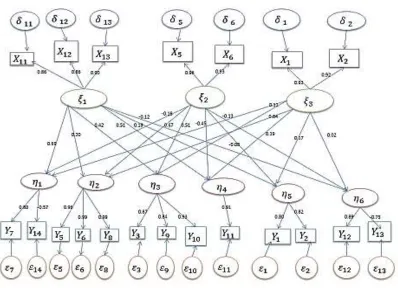
Technically, SEMs hold one or more linear regressions that explain how endogenous structures are determined upon exogenous structure. That means, in SEM the focus is in terms of measurement of variables that define just how theoretical (indirect) structures depend on observed variables when assuming causality relationship between indirect variables. Path analysis (PA) and confirmatory factor analysis (CFA) are special types of SEM. PA examines how independent variables are statistically related to a dependent variable. Moreover, PA can allow causal interpretation of statistical dependencies and most importantly, PA allows for the examination of how the data fits to a theoretical model. PA enables us both to draw a path diagram based on the theory and to conduct one or more regression analysis (see Figure 1 and 2).
The estimation process in SEM involves different techniques, which include maximum likelihood commonly used by software. It assumes either multivariate normality or generalized least square of robust estimators.
SEM using J𝑜̈reson in linear structural relations (LISREL) notations as presented by Bentler and Weeks (1980) follows:
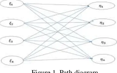
Figure 1. Path diagram
Figure 1 presents a path diagram for a linear SEM that provides solutions to the problem of hunger in Sub-Saharan Africa (SSA) by increasing food production when using the relationship between the exogenous and endogenous variables.
Most often, PA provides a diversity of set of relationships that can be developed among the variables. However, some of these variables are similar. Therefore, there is a need of a more advanced technique (or method) that allows us to reduce a large number of variables into a small number. Factor analysis (FA) serves this purpose. FA is a multivariate statistical method for reducing large numbers of variables to fewer underlying dimensions. This method involves grouping of similar variables into dimensions. This process is used to identify latent variables or constructs. Most often, factors are rotated after extraction. FA has several different rotation methods, and some of them ensure that the factors are orthogonal (i.e. uncorrelated), which eliminates problems of multicollinearity in regression analysis. There are many techniques of FA with principal component analysis (PCA) being the most used followed by the exploratory factor analysis (EFA). PCA is used if the components can be derived or/and summarized. It has been used by many researchers in medical science, education, social science and many other related fields (Wang and Staver, 2001; Bolt et al., 2018). However, EFA is used if the variables have unmeasured variables. It is not as popular as PCA. In this paper, we integrate FA into SEM in order to provide an optimal and cost effective model that explains better the key factors in the food production system.
3. Methodology
The current approach of SEM is more restrictive since it specifies the latent variables that are involved in the analysis and creates the theoretical relations between the variables. There is a huge diversity of set of relationships that could be developed among the variables. The variability of set of relationships point to inconsistent conclusions about the level at which a model truly is equivalent to the observed data. Therefore, a variety of the path diagram are oftentimes utilized. We present a more reliable approach that provides a guideline on how to evaluate the suitability of a given SEM. Researchers in agriculture sector use all possible variables that might be identified for a set data, but using factor analysis through the PCA, researchers will be able to use the most important variables in the model. SEM, commonly applied in many fields is introduced in the agriculture field.
We outline necessary steps to take in producing SEM using factor analysis after obtaining provisional factors via principal component analysis (PCA) as follow:
(i) Screen the data for suitability through testing;
(ii) Apply PCA on correlation matrix to obtain provisional factors when the test in Step (i) is statistically significant. Using the Factor analysis (FA), calculate the communalities accounting for pre-set proportion of total variation;
(iii) Determine the number of principal components to retain and rotate to obtain orthogonality;
(iv) Interpret the new variables (FAs) based on factor loading for each variable;
(v) Consider rotating the factors to attain orthogonality. Thus, final factors are orthogonal;
(vi) Determine the component score coefficient matrix for the possible models.
Estimation of parameters in SEM is by maximum likelihood method. It provides estimates for the linear equations that reduce the deviation between the observed and the proposed model. We incorporate the selected Factors to a number of SEMs and then test for different inter-associations among the latent variables. The correlations between the latent (unobserved) variables and latent (observed) variables were equivalent to factor loading in principal component analysis. The general structural equation model as given in Equation (1a) is equivalent to Equation (2) summarized as
𝜂 = 𝛽+𝜂 +Σ𝜉 + 𝜁, (2)
where 𝜂 = (
𝜂1 𝜂2 𝜂3 𝜂4
), 𝛽+ = ( 0 0
𝛽12 0
𝛽13 𝛽14 𝛽23 𝛽24
0 0 0 𝛽34
0 0 0 0
), Σ=Γ = ( 𝛿11 𝛿21
𝛿12 𝛿22
𝛿13 𝛿14 𝛿23 𝛿24 𝛿31 𝛿32 𝛿33 𝛿34 𝛿41 𝛿42 𝛿43 𝛿44
) , 𝜉 = ( 𝜉1 𝜉2 𝜉3 𝜉4
)
and 𝜁 = ( 𝜁1 𝜁2 𝜁3 𝜁4
)
These structures of random vectors and parameter matrices are used in the data analysis.
3.2 Data analysis
only be estimated from the observed core factors. These factors are identified through the PCA and FA procedures.
Consider data from the FAO database http://faostat3.org/home/E from 2015 across 45 African countries. The variables are given in Table 1 with the LISREL notations according to J𝑜̈reskog (2000).
Table 1: Crop components classified into three vital factors (crop, livestock and contributors) with various factor levels and denoted by LISREL
Components Description
of variables
LISREL notations
Crop Banana 𝑌1
Beans 𝑌2
Cassava 𝑌3
Rice 𝑌4
Groundnut 𝑌5
Maize 𝑌6
Sugar cane 𝑌7 Vegetables 𝑌8 Cereals 𝑌9 Fruits 𝑌10 Livestock Cattle and
Buffaloes
𝑌11
Pigs 𝑌12
Poultry 𝑌13 Sheep and
Goats
𝑌14 Contributors Fertilizer
(Factor 1)
Nitrogen 𝑋1 Phosphate 𝑋2 Trade
(Factor 2)
Export values 𝑋3 Import values 𝑋4 Labour
(Factor 3)
Rural 𝑋5
Urban 𝑋6
Land (Factor 4)
Arable 𝑋7 Permanent 𝑋8 Water
(Factor 5)
Rainfall 𝑋9 Irrigated land 𝑋10 Energy used
(Factor 6)
Electricity 𝑋11 Diesel 𝑋12 Transport 𝑋13
Suppose we denote crop components Y1, Y2, . . .,Y10, livestock components Y11, Y12, . . .,Y14 and contributors components X1, X2, . . .,X13.
into crop production, livestock and contributors factors dimensions and make inference about stable estimate parameters for the solutions to the problem of hunger and life of human being at the extreme menace. We used the PCA approach to determine direct and indirect variables.
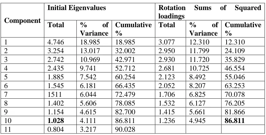
The correlation matrix is used to determine the variables that were the most strongly correlated with each component. This screening of variables reduced the number of highly correlated variables from 25 to 10 new independent variables as indicated in Table 2. The retained variables explain much of the total variation in the variable of interest is explained by each component, as this cannot be performed in multiple regressions. The results of PCA determined the levels at which the variables were measured. The variables with the highest sample variances were among the few components taken as each variable received its particular weight in the analysis. To receive equal weight in the analysis we have then standardized variables before carrying out the PCA (performing PCA on a correlated matrix). Table 2 shows the number of components and the eigenvalues (initial and rotation eigenvalues).
Table 2: Screening of different variables through PCA based on the total variance explained
Component
Initial Eigenvalues Rotation Sums of Squared loadings
Total % of
Variance
Cumulative %
Total % of Variance
Cumulative %
1 4.746 18.985 18.985 3.077 12.310 12.310 2 3.254 13.017 32.002 2.950 11.799 24.109 3 2.742 10.969 42.971 2.930 11.720 35.829 4 2.435 9.741 52.712 2.681 10.725 46.554 5 1.885 7.542 60.254 2.123 8.492 55.046 6 1.545 6.181 66.435 2.052 8.207 63.253 7 1511 6.044 72.479 1.706 6.825 70.078 8 1.402 5.606 78.085 1.532 6.127 76.205 9 1.154 4.615 82.700 1.415 5.661 81.866
10 1.028 4.111 86.811 1.236 4.945 86.811
11 0.804 3.217 90.028
Extraction Method: Principal Component Analysis
From Table 2, about 87% of the total variation is accounted for by 10 out of 25 original variables. Thus, we rotate the 10 principal components using FA to attain orthogonality.
3.3 Illustrative Example on Agricultural Data Analysis using SEMs
use of more advanced agricultural technology. We have used food production to display the values of this modelling method.
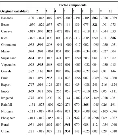
In this section, the proposed technique is implemented using a real-life example based on food production in order to show how the newly proposed model prevails on the existing models. In this illustrative example, most valuable crops, livestock’s products and the contributor’s factors in the SSA are given in column 1 of Table 1. PCA procedure allows for reduction of dimension of the original variables into a few number of the principal components as variables explaining most of the variation in the data set. These principal components are represented by component 1 to 10 as given in Table 3. The bold values are the highest correlations between the original variables and the components in the array.
Table 3: The rotate component matrix
Original variables
Factor components
1 2 3 4 5 6 7 8 9 10
Bananas .100 -.045 .049 -.099 -.009 -.191 -.105 .802 -.038 -.039 Beans -.050 -.029 .057 -.076 .114 .139 .075 .821 -.001 .073 Cassava -.017 .040 .872 -.072 .089 .012 -.019 .114 -.044 .053 Rice -.072 -.024 .090 .000 -.038 -.117 -.005 .050 -.031 .886
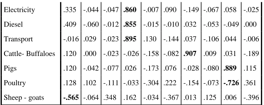
Electricity .335 -.044 -.047 .860 -.007 .090 -.149 -.067 .058 -.025 Diesel .409 -.060 -.012 .855 -.015 -.010 .032 -.053 -.049 .000 Transport -.016 .029 -.023 .895 .130 -.144 .037 -.106 .044 -.006 Cattle- Buffaloes .120 .000 -.023 -.026 -.158 -.082 .907 .009 .031 -.189 Pigs .120 -.042 -.077 .026 -.173 .076 -.028 -.080 .889 .115 Poultry .128 .102 -.111 -.033 -.304 .222 -.154 -.073 -.726 .361 Sheep - goats -.565 -.064 .348 .162 -.034 -.367 .013 .125 .006 -.396 The dominance variables explaining each of the 10 factors accounting for 87% of the total variation are outlined below:
Factor 1 --- Sugar cane, Import, Irrigated and Sheep - Goat Factor 2 --- Groundnut, Maize, and Vegetables
Factor 3 --- Cassava, Cereals, and Fruits Factor 4 --- Electricity, Diesel, and Transport Factor 5 --- Rural and Urban
Factor 6 --- Nitrogen and Phosphate Factor 7 --- Rainfall and Cattle - Buffalos Factor 8 --- Bananas and Beans
Factor 9 --- Pigs and Poultry Factor 10 ---Rice.
The test for normality of the variables in each of the observed indicator for endogenous and exogenous variables is validated as shown in Tables 4 and 5.
Table 4: Test for normality for endogenous variable
Observation Factor 1 Factor 2 Factor 3 Factor 4 Factor 5 Factor 6
Chi-square 88.942 263.882 113.417 18.676 8.068 6.940
Degrees of freedom 10 3 6 1 1 1
p-value 0.000 0.000 0.000 0.000 0.005 0.008
Table 5: Test for normality for exogenous variables
Observation Factor 1 Factor 2 Factor 3
Degrees of freedom 3 1 1 p-value 0.000 0.000 0.000
The variables were normally distributed since 𝑝 − 𝑣𝑎𝑙𝑢𝑒 is less than 0.05. Therefore, the maximum likelihood estimation can be used. The general linear SEM is given in Equations (1a), (1b) and (1c) (See Tables 6 and 7). The latent endogenous and exogenous models are the highly correlated of the factors load in which the measurement model is obtained by the maximum likelihood. The model fit was the result for the goodness-of-fit statistical tests that explain the discrepancy between latent and unobserved variables. In this practice, the model fits well the data as this indicated that no important paths have been omitted from the model.
After estimating the endogenous and exogenous latent measurement model separately, a joint model that includes altogether latent model can now be estimated (Figure 2).
Since latent variables are observed, the measurement is obtained indirectly through the latent endogenous and exogenous variables. The latent unobserved variables are represented as ellipses and the latent observed variables are represented as rectangles and because we cannot measure or estimate perfectly the unknown factors or parameters, we can only measure with error and therefore, the errors terms were associated with each of the latent observed variables as they form part of the overall model. The error terms are also represented as ellipse (Figure 2).
Figure 2. Conceptual path diagram for the structural model
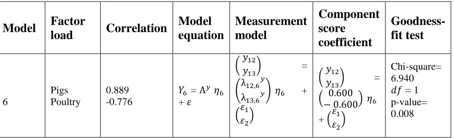
Table 6 presents the endogenous variables under different models based on the factor loadings obtained from rotated provisional factors. The model equations, measurement model parameters and associated score components, in addition to goodness of fit test statistics are also included
Model Factor
load Correlation
Model equation Measurement model Component score coefficient Goodness-fit test 1 Sugar Export Import Irrigation Sheep & goats 0.804 0.707 0.659 0.775 0.565
𝑌1 = Λ𝑦𝜂1
+ 𝜀 ( 𝑦7 𝑦14 𝑥3 𝑥4
𝑥10)
=
( λ71𝑦
λ14,1𝑦
λ31𝑦
λ41𝑦
λ10,1𝑦)
𝜂1 +
( 𝜀1
𝜀2
𝜀3
𝜀4
𝜀5)
( 𝑦7
𝑥3
𝑥4
𝑥10
𝑦14)
= ( 0 0.649 0.445 0 0 ) 𝜂1 + ( 𝜀1 𝜀2 𝜀3 𝜀4
𝜀5)
Chi-square= 8.018 𝑑𝑓 = 4 p-value= 0.005 2 Groundnut Maize Vegetable 0.960 0.990 0.993
𝑌2 = Λ𝑦𝜂2
+ 𝜀 ( 𝑦5 𝑦6 𝑦8 ) = ( λ52𝑦
λ62𝑦
λ82𝑦
) 𝜂2 +
( 𝜀1 𝜀2 𝜀3 ) ( 𝑦5 𝑦6 𝑦8 ) =
(0.0550.936 0.013) 𝜂2 +
( 𝜀1 𝜀2 𝜀3 ) Chi-square= 0.637 𝑑𝑓 = 2 p-value= 0.000 3 Cassava Cereals Fruits 0.872 0.843 0.933
𝑌3 = Λ𝑦𝜂3
+ 𝜀 ( 𝑦3 𝑦9 𝑦10 ) = ( λ33𝑦
λ93𝑦
λ10,3𝑦
) 𝜂3 +
( 𝜀1 𝜀2 𝜀3 ) ( 𝑦3 𝑦9 𝑦10 ) =
(0.1520.186 0.688) 𝜂3 +
( 𝜀1 𝜀2 𝜀3 ) Chi-square= 15.49 𝑑𝑓 = 2 p-value= 0.000
4 Rainfall
Cattle
0.868 0.907
𝑌4 = Λ𝑦𝜂4
+ 𝜀
( 𝑦 𝑋9
11) =
(λ94
𝑦
λ11,4𝑦) 𝜂4 +
(𝜀𝜀1
2)
( 𝑋9
𝑦11) =
(0.5600.560) 𝜂4 +
(𝜀𝜀1
2)
Chi-square= 16.68 𝑑𝑓 = 1 p-value= 0.000
5 Banana
Beans
0.802 0.821
𝑌5 = Λ𝑦𝜂5
+ 𝜀
( 𝑦 𝑦1
2) =
(λ15
𝑦
λ25𝑦) 𝜂5 +
(𝜀𝜀1
2)
( 𝑦 𝑦1
2) =
(0.5940.594) 𝜂5 +
(𝜀𝜀1
2)
Model Factor
load Correlation
Model equation Measurement model Component score coefficient Goodness-fit test 6 Pigs Poultry 0.889 -0.776
𝑌6 = Λ𝑦𝜂6
+ 𝜀
( 𝑦 𝑦12
13) =
(λ12,6
𝑦
λ13,6𝑦) 𝜂6
+
(𝜀𝜀1
2)
( 𝑦 𝑦12
13) =
( 0.600− 0.600) 𝜂6
+ (𝜀𝜀1
2)
Chi-square= 6.940 𝑑𝑓 = 1 p-value= 0.008
Table 7: The exogenous descriptions model
Mode l Factor load Correlatio n Model equatio n Measuremen t model Componen t score coefficient Goodness -fit test 1 Electricit y Diesel Transport 0.860 0.855 0.895
𝑋1 = Λ𝑥𝜉1
+ 𝛿 ( 𝑋11 𝑋12 𝑋13 ) = ( λ33𝑥
λ93𝑦
λ10,3𝑥
) 𝜉1 +
( 𝛿 1
𝛿 2
𝛿 3
) ( 𝑋11 𝑋12 𝑋13 ) =
(0.3760.582 0.057) 𝜉1 +
( 𝛿 1
𝛿 2
𝛿 3
)
Chi-square= 15.49 𝑑𝑓 = 2 p-value= 0.000
2
Rural
Urban 0.961 0.934
𝑋2 = Λ𝑥𝜉2
+ 𝛿
( 𝑋 𝑋5
6) =
(λ52𝑥
λ62𝑥) 𝜉2
+
( 𝛿 𝛿 1
2)
( 𝑋 𝑋5
6) =
(0.5130.513) 𝜉2 +
( 𝛿 1
𝛿 2)
Chi-square= 69.64 𝑑𝑓 = 1 p-value= 0.000 3 Nitrogen Phosphat e 0.919 0.922
𝑋3 = Λ𝑥𝜉3
+ 𝛿
( 𝑋𝑋1
2) =
(λ1,3
𝑥
λ2,3𝑥) 𝜉3
+
( 𝛿 𝛿 1
3)
( 𝑋𝑋1
2) =
(0.5240.057) 𝜉3 +
(𝛿 1
𝛿 3)
Chi-square= 48.16 𝑑𝑓 = 1 p-value= 0.000
variables” given that their impact depends stochastically on the operation system of food that solves the problem of hunger in the SSA. The arrows between these variables indicate that one variable was a cause of the other variable and 𝜀𝑖(𝑖 = 1, 2, …, 6) and 𝛿𝑖 (𝑖 = 1, 2, and 3) are random variables that are assumed to be multivariate normal distribution. This means the expectation of the vector 𝜀 or 𝛿 is assumed to be equal to zero. For instance, the variance-covariance matrix of 𝜀 or 𝛿 was assumed to be zero and the 𝐶𝑜𝑣 ( 𝜀1, 𝜀2 ) = 𝐶𝑜𝑣 ( 𝜀2, 𝜀3 ) = ... = 𝐶𝑜𝑣 ( 𝜀𝑖, 𝜀𝑗 ) = 0, where 𝑖 = 1, 2, ..., n and j = 1, 2, ..., m.
Using the path diagram, the absence of curved arrows between the variables in 𝜀 or 𝛿 indicated that the covariance matrix equals to zero as assumed above.
This is the result of the power of the exploratory properties of factor analysis by showing strong indication against orthogonality solutions in this complexity of data. Therefore, the six-measurement model in matrix notation for the exogenous model equivalent to the path diagram 2 represented by Equation (1b) is then given by
( 𝑦1 𝑦2 𝑦3 𝑦4 𝑦5 𝑦6 𝑦7 𝑦8 𝑦9 𝑦10 𝑦11 𝑦12 𝑦13 𝑦14)
=
(
0.000 0.000 0.000 0.000 0.594 0.000 0.000 0.000 0.000 0.000 0.594 0.000 0.445 0.000 0.152 0.000 0.000 0.000 0.000 0.000 0.000 0.000 0.000 0.000 0.000 0.055 0.000 0.000 0.000 0.000 0.000 0.936 0.000 0.000 0.000 0.000 0.000 0.000 0.000 0.000 0.000 0.000 0.000 0.013 0.000 0.000 0.000 0.000 0.000 0.000 0.186 0.000 0.000 0.000 0.000 0.000 0.688 0.000 0.000 0.000 0.000 0.000 0.000 0.000 0.000 0.000 0.000 0.000 0.000 0.000 0.000 0.600 0.000 0.000 0.000 0.000 0.000 −0.60 0.649 0.000 0.000 0.000 0.000 0.000)
( 𝜂1 𝜂2 𝜂3 𝜂4 𝜂5 𝜂6)
+ ( 𝜀1 𝜀2 𝜀3 𝜀4 𝜀5 𝜀6 𝜀7 𝜀8 𝜀9 𝜀10 𝜀11 𝜀12 𝜀13 𝜀14)
(3)
In the same way, the exogenous measurement model represented by Equation (1c) is given by ( 𝑋1 𝑋2 𝑋3 𝑋4 𝑋5 𝑋6 𝑋7 𝑋8 𝑋9 𝑋10 𝑋11 𝑋12 𝑋13)
= ( 0.376 0 0 0 0 0 0 0 0 0 0 0.582 0 0 0 0.513 0.513 0 0 0 0 0 0.057 0 0 0 0 0 0 0 0 0 0.524
0 0 0
0 0 0.057)
( 𝜉1 𝜉2 𝜉3 ) + ( 𝛿 1 𝛿 2 𝛿 3 𝛿 4 𝛿 5 𝛿 6 𝛿 7 𝛿 8 𝛿 9 𝛿 10 𝛿 11 𝛿 12 𝛿 13)
(4)
Table 8: The parameters estimates and measurement model matrices Β = ( 0 0 0 0 0.527 0 0 0
0.098 0.008 0.094 −0.025 −0.196 0.265 −0.102 0.066 0 0.217 0.548 −0.634
0 0 −0.454 0.207 0 0 0 0 0 0.244 0 0 0 0 0 0 )
𝜂 = ( 𝜂1 𝜂2 𝜂3 𝜂4 𝜂5 𝜂6)
Γ = ( 0.707 −0.087 0.384 0 0.673 −0.036 −0.141 0
0.193 0 0 0 0.761 0 0 0 −0.567 0 0 0 0 0 0 0
0 0 0 0 0 0
0 0 0 0 0 0 )
𝜁 = ( 𝜁1 𝜁2 𝜁3 𝜁4 𝜁5 𝜁6)
𝜉 = ( 𝜉1 𝜉2 𝜉3 𝜉4 𝜉5 𝜉6)
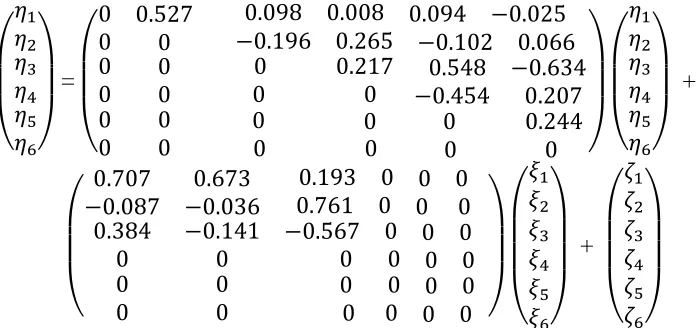
The structural model estimated with the class of the linear model as given in Equation (2) is equivalent to
( 𝜂1 𝜂2 𝜂3 𝜂4 𝜂5 𝜂6)
= ( 0 0 0 0 0.527 0 0 0
0.098 0.008 0.094 −0.025 −0.196 0.265 −0.102 0.066 0 0.217 0.548 −0.634
0 0 −0.454 0.207 0 0 0 0 0 0.244 0 0 0 0 0 0 )(
𝜂1 𝜂2 𝜂3 𝜂4 𝜂5 𝜂6)
+ ( 0.707 −0.087 0.384 0 0.673 −0.036 −0.141 0
0.193 0 0 0 0.761 0 0 0 −0.567 0 0 0 0 0 0 0
0 0 0 0 0 0
0 0 0 0 0 0 )(
𝜉1 𝜉2 𝜉3 𝜉4 𝜉5 𝜉6)
+ ( 𝜁1 𝜁2 𝜁3 𝜁4 𝜁5 𝜁6)
Having the latent scores for 𝜂1,𝜂2, 𝜂3, 𝜂4, 𝜂5 and 𝜂6, and 𝜉1, 𝜉2 and 𝜉3, we can use the information from the model to compare the productivity level for all the identified components. Based on this information, Figure 2 entails that a primary crop production level was simultaneously controlled by the support of livestock (using manure) and the contributor’s factors. The SEMs obtained extract more information about the food production then when using a single linear model for instance maize. In so doing with latent scores, we were able to estimate a single linear equation by using ordinary least squared (OLS) through 𝜂1 as endogenous variable. This procedure generates the equation 𝜂1= - 0.0479𝜉1 – 0.0182 𝜉2 + 0.404 𝜉3 . For illustration of the model, this suggested that 𝜂1 was a linear function of 𝜉1 , 𝜉2 and 𝜉3 and as a result, the components units can be ranked either on the basis of 𝜂1 or - 0.0479 𝜉1 – 0.0182 𝜉2 + 0.404 𝜉3.
diverse set of linear equations describing the relationships that define a certain pattern when using variance-covariance matrix.
The results were as amazingly natural as the correlations between latent (unobserved) variables and observed variables were found highly correlated (all above 0.80) and in positive direction except Y (poultry) that was negatively strong (- 0.73) and Y representing sheep and goats (− 0.57) that was acceptable relationship. By contrast, the relationship between the latent (unknown) variables was positively weak but statistically significant. Given these patterns, it appears both a direct and indirect effect between exogenous and endogenous variables. The six endogenous variables derived from the diverse type of crop and kind of livestock affect mutually the three direct cause-factors exogenous: energy, labour and fertilizer as this is likely to maintain claims by revealing how well it is organized. Conversely, the energy used as a factor, labour and fertilizer types were likely to be exceptionally confident, as these factors were key feature to create more productivity of crop and conserve healthy livestock.
4. Conclusion and Recommendations
SEM and path analysis have been used in many fields of science to solve complex problems. This paper introduced the use and application of SEM in agricultural field in an explicit and illustrative manner. Path analysis is a technique to be used in agricultural studies since it helps to focus on the key activities of food production and how they all fit together. SEM and path analysis being statistical techniques of making decision, they also have their own strength and limitations. The best method should be the one addressing the purpose of the research. We have assumed that there is a causal structure among a set of latent variables, therefore SEM technique applied to food production has validated that the livestock’s products and crop in its diversities are likely to be integrated. The results also revealed that factors such as energy, labour and fertilizer are anticipated to make positive contributions to the increase of food production in SSA. Multiple factors influence greater food productivity returns over the viewing platform, including new and faster technology adoption of small-scale producers. Despite the confirmation of SEM, improvement and important gaps remain. To close current yield food production gaps represent the greatest challenges and uncertainties facing SSA.
Acknowledgements
The authors thank the University of South Africa and the Master and Doctoral Research Support Programme (MDSP) for their support.
References
1. Ali, F., Rasoolemanesh, S.M., Sarstedt, M., Ringle, C. M., and Ryn, K. (2017). Partial Least Squares Structural Equation modeling. Handbook of Market Research pp 1-40.
3. Bentler, P.M. and Chou, C.P. (1986). Practical Issues in Structural Modelling. Sage journals. Los Angeles.
4. Bentler, P.M. and Weeks, D.G. (1980). Linear Structural Equations with Latent Variables. Psychometrika, 45(3), 289-308.
5. Bolt, T., Prince, E.B., Nomi, J.S., Messinger D., llabre, M.M. and Uddin, L.Q. (2018). Combining region-and network-level brain-behavior relationships in a Structural equation model. NeuroImage, 1656 158-16.
6. Bielby, W.T. and Hauser, R.M. (1977), Structural Equation Models. Annual Review of Sociology, 3, 137-161.
7. Goodboy, A.K., and Kline, R B. (2017). Statistical and Practical Concerns with Published Communication Research featuring Structural Equation Modeling. Communication Research Reports, 34, 1, 68-77.
8. Hair, J. F., Hult, G.T.M., Ringle, C.M., Sarstedt, M. and Thiele, K.O. (2017). Mirror, Mirror on the wall: a Comparative Evaluation of Composite-based Structural Equation Modeling Methods. Journal of the Academy of Marketing Science, 45, 616-632.
9. Henseler, J. (2017). Briging Design and Behavioral Research with variance-based Structural Equation Modeling. Journal of Advertising, 46, 178-192.
10. Jöreskog, K.G. (2000). “Latent variable Scores”. Available at http://www.ssicentral.com/Liserl /advancedtopics.html.
11. Kaufmann, L. and Gaeckler, J. (2015). A structural review of partial least squares in supply chain management research. Journal of Purchasing and Supply Management, 21(4), 259-272.
12. Lamb, E., Shirtliffe, S. and May, W. (2010). Structural Equation Modeling in the plant sciences: An example using yield components in oat. Canadian Journal of Plant Sciences, 91(4), 603-619.
13. Lee, L., Petter, S., Fayard, D., and Robinson, S. (2011). On the use of partial least squares path modeling in accounting. Research International Journal of Accounting Information Systems, 12(4), 305-328.
14. Mwichabe, S. (2013). The African Agrarian Ideology and food security challenge in Sub-Saharan Africa. Development, 56(3), 412-420.
15. Nitzl, C. (2016). The use of Partial least squares Structural equation modelling (PLS=SEM) in Management Accounting Research: direction for future theory development. Journal Accounting Literature, 37, 19-35.
16. Peng, D.X. and Lai, F. (2012). Using partial least squares in Operation Managers research: A practical guideline and summary of past research. Journal of Operations Management, 30(6), 467-480.
18. Steenkamp, J.B.E.M., and Baumgartner, H. (2000). On the Use of Structural equation models for Marketing modelling. International Journal of Research in Marketing, 17, 195-202.
19. Singh, K., Granville, M. and Dika, S. (2002). Mathematics and Science achievement: Effects of motivation, interest, an academic engagement. The journal of Education Research, 95, 323-332.
20. Sosik, J.J., Kahai, S.S. and Piovoso, M.J., (2009). Silver bullet or Voodoo Statistics? A primer for using the partial least squares data analytic technique. Group and Organization Research Group and Organization Management, 34(1), 5-36.
21. Raykov, T. and Marcoulides G. A. (2000). First Course in structural equation modeling. The Amazon Book Review.
22. Richter, N. F., Sinkovics, R.R., Ringle, C. M., and Schlagel, C. (2016). A critical look at the use of Structural Equation Model in International Business Research. International Marketing Review, 33(3), 376-404.
23. Wang, J. and Staver J.R., (2001). Examining relationships between factors of Science education and student career aspiration. The Journal of Educational Research, 94, 312-319.