Confidence Intervals for the Reciprocal of a Normal Mean with a Known Coefficient of Variation and a Restricted Parameter Space

(1)

Known Coefficient of Variation and a Restricted Parameter Space

Wararit Panichkitkosolkul

Department of Mathematics and Statistics Thammasat University, Phathum Thani, Thailand [email protected]

Abstract

The natural parameter space is known to be restricted in many real applications such as engineering, sciences and social sciences. The confidence interval derived from the classical Neyman procedure is unsatisfactory in the case of a restricted parameter space. New confidence intervals for the reciprocal of a normal mean with a known coefficient of variation and a restricted parameter space are proposed in this paper. A simulation study has been conducted to compare the performance of the proposed confidence intervals.

Keywords: Estimation, Normal distribution, Central tendency, Simulation.

Mathematics subject classification 62F25

1. Introduction

The reciprocal of a normal mean, defined by 1 ,

 _ 

where  is the population mean, is widely used in many areas, such as experimental nuclear physics, biological sciences, agriculture and econometrics. For example, Lamanna et al. (1981) studied charged particle momentum, _p1

(2)

terms of coverage probability. However, the approximate confidence interval is very easy to calculate compared with the exact confidence interval.

Although statistical inference is studied in a natural parameter space, the parameter space is restricted in several real applications, such as engineering, sciences and social sciences. For example, the blood pressure of patients or the weight of a human body are restricted or bounded. Furthermore, Mandelkern (2002) indicated the importance of statistical inference where the parameter space is known to be restricted. Additionally, he gave the example that the classical Neyman procedure is unsatisfactory in the case of a restricted parameter space. The main reason is that the information regarding the restriction is simply ignored. The other related works are Feldman and Cousins (1998) and Roe and Woodroofe (2001). Although research has been done on confidence intervals for the reciprocal of a normal mean, the confidence intervals for the reciprocal of a normal mean with a restricted parameter space have not been the subject of much study. Therefore, it would be of significant interest to develop confidence intervals for the reciprocal of a normal mean that include additional information on the population mean being restricted in order to improve the accuracy of the confidence interval. Motivated by the recent work of Panichkitkosolkul (2017), we propose confidence intervals for the reciprocal of a normal mean with a known coefficient of variation and a restricted parameter space in this paper.

The structure of this paper is as follows: Section 2 reviews two confidence intervals for the reciprocal of a normal mean with a known coefficient of variation. Confidence intervals for the reciprocal of a normal mean with a known coefficient of variation and a restricted parameter space are proposed in Section 3. The performance of all confidence intervals is investigated through a Monte Carlo simulation study in Section 4. We then conclude this paper in Section 5.

2. Confidence Intervals for the Reciprocal of a Normal Mean with a Known Coefficient of Variation

In this section, we review the confidence intervals for the reciprocal of a normal mean with a known coefficient of variation proposed recently by Wongkhao et al. (2013) and Panichkitkosolkul (2017). The exact and the approximate confidence intervals for the reciprocal of a normal mean with a known coefficient of variation are discussed.

The theorem and corollary proposed by Wongkhao et al. (2013) are reviewed and used to construct the exact confidence interval for .

Theorem 1. (Wongkhao et al., 2013) Let X₁,...,X_n be a random sample of size n from a

normal distribution with mean  and variance 2

.

 The estimator of  is ˆ 1

X

_  _where

1

1 . n

i i

X n X





The expectation of ˆ and ˆ2

when a coefficient of variation,    / is

known, are respectively

2

1 (2 )! ˆ

( ) 1

2 !

k

k k

k E

k n



  



 _ _ 

 

  _ _

   







(3)

  2 2 2 1 (2 1)! ˆ ( ) . 2 ! k k k k E k n          _ _  





Proof of Theorem 1 See Wongkhao et al. (2013).

From (1), lim ( )ˆ

nE   and ˆ

( / ) ,

E w  where

2 1 (2 )! 1 . 2 ! k k k k w k n        _ _  



Therefore, the

unbiased estimator of  is ˆ /_w₍_wX_{) .}1

Corollary 1. From Theorem 1, ˆ 2 2

var( )    / .n

Proof of Corollary 1 See Wongkhao et al. (2013).

From the central limit theorem, we will use the fact that, ˆ (0,1). ˆ

var( )

Z   N





 Based on

Theorem 1 and Corollary 1, we get

2 2 ˆ / (0,1). / w Z N n              

Therefore, the 100(1)% exact confidence interval for  based on Equation (2) is

1 2 2 1 2 2

1 / 2 1 / 2

( ) / , ( ) / ,

Exact

CI  _ wX  z  nX wX  z  nX _

where 2 1 (2 )! 1 2 ! k k k k w k n        _ _  



and z1/ 2 is the 100(1/ 2) percentile of the standard

normal distribution.

Next, the following theorem suggested by Panichkitkosolkul (2017) is shown to find the approximate confidence interval for .

Theorem 2. Let X₁,...,X_n be a random sample of size n from a normal distribution with

mean  and variance 2

.

 The estimator of  is ˆ 1

X

 _ 

where 1

1 . n

i i

X n X





The

approximate expectation and variance of ˆ when a coefficient of variation,    / is known, are respectively

2 1 ˆ

( ) 1

E n       _  _

  (3)

and

2 2 ˆ

var( ) .

n

 

  (4)

Proof of Theorem 2 See Panichkitkosolkul (2017).

It is clear from Equation (3) that ˆ is asymptotically unbiased



lim ( )ˆ



nE  and ˆ

( / ) ,

E  v  where 2

1 / .

(4)

From Equation (4), ˆ is consistent



lim var( )ˆ 0 .



n   Then, the central limit theorem and Theorem 2 are applied and we get,

2 2 ˆ /

(0,1). /

v

Z N

n

 

 

 

Therefore, it is easily seen that the (1)100% approximate confidence interval for  is

1 2 2 1 2 2

1 / 2 1 / 2

( ) / , ( ) / ,

Approx

CI  _ vX  z  nX vX  z  nX _

where 2

1 /

v  n and z₁___{/ 2} is the 100(1/ 2) percentile of the standard normal distribution.

3. Confidence Intervals for the Reciprocal of a Normal Mean with a Known Coefficient of Variation and a Restricted Parameter Space

Confidence intervals for the mean of a normal distribution with restricted parameter space were derived by Wang (2008). Following the method proposed by Wang (2008), we present confidence intervals for the reciprocal of a normal mean with a known coefficient of variation when the population mean is restricted.

The true value of a parameter of interest is usually unknown. However, parameter space is often known to be restricted and the bounds of parameter space are known. We denote

1

m and m₂ as the lower bound and the upper bound of the parameter space. When the parameter space is known to be restricted to the interval (m m1, 2), it is widely accepted

that the confidence interval for a parameter  is the confidence interval of the intersection between the interval (m m₁, ₂) and L U, , where L and U are the lower

and upper limits of the confidence interval for . Therefore, the confidence interval for

 when the parameter space is restricted, denoted as CIB, is defined as

1 2

max( , ), min( , ) . B

CI  _ m L_ m U_ _ (5)

Four possible confidence intervals in (5) are as follows:

1) if m₁L and m2U then CIB is reduced to CIB m U1, .

2) if m₁L and m2U then CIB is reduced to CIB



m m1, 2



. 3) if m₁L and m2U then CIB is reduced to CIB L U, .

4) if m₁L_ and m₂U_ then CI_B is reduced to CI_B L m, ₂.

When the parameter space of the population mean is (m m1, 2), straightforward calculation can show that the reciprocal of a normal mean is also restricted as follows:

1 2

m   m

 1 1 1

2 1

(5)

According to Wang (2008) and Niwitpong (2013), the proposed confidence intervals for  with a restricted mean are given by



1





1



2 1

max , , min , ,

CI   m L m U 

where L_ and U_ are the lower and upper limits of the confidence intervals for , respectively. In addition, the exact and approximate confidence intervals for  reviewed in the previous section are used in order to obtain confidence intervals for  when the population mean is restricted.

4. Simulation Results

The performances of the confidence intervals for the reciprocal of a normal mean with a known coefficient of variation and a restricted parameter space derived in the previous section were investigated through simulation studies in this section. A simulation was conducted using the R statistical software (Ihaka and Gentleman, 1996) version 3.3.2. The estimated coverage probabilities and expected lengths of two confidence intervals with unrestricted and restricted population means are demonstrated in Tables 1-6. The sets of normal data were generated with  = 0.1, 0.2, 0.5, 1, 5 and 10, and the coefficient of variation  = 0.05, 0.10, 0.20, 0.33 and 0.50. The sample sizes were set at n = 10, 20, 30, 50 and 100. The parameter space of the population mean was set to the interval (0.9 / , 0.11/ ).  The number of simulation runs was 10,000 and the nominal confidence level 1 was fixed at 0.95.

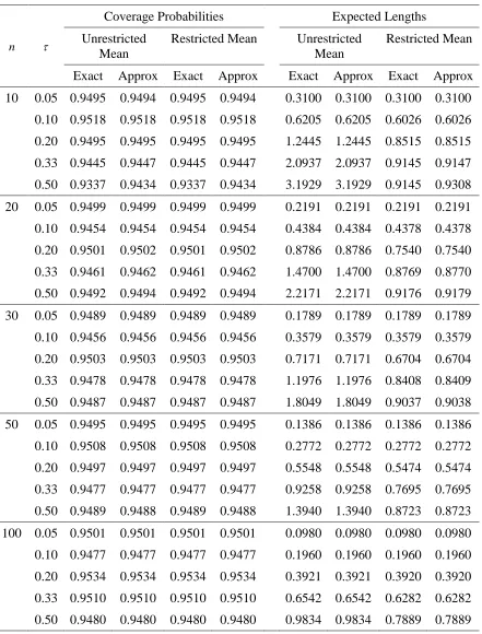
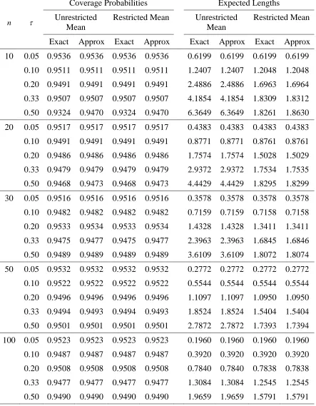
In the simulation study, the estimated coverage probabilities of the confidence intervals with a restricted population mean are the same as those of the confidence intervals with an unrestricted population mean. Additionally, all confidence intervals have estimated coverage probabilities close to the nominal confidence level in most situations. The estimated coverage probabilities of all the confidence intervals do not increase or decrease according to the values of  and n. The confidence intervals with a restricted population mean have shorter expected lengths than those of the confidence intervals with an unrestricted population mean when the sample sizes are not too large and the values of  are not too small.

5. Conclusion

(6)

Appendix: Source R code for all confidence intervals

cal.w <- function(tao,n)

{

temp <- rep(0,50) for (k in 1:50) {

temp[k] <- (factorial(2*k)/((2^k)*factorial(k)))*(((tao^2)/n)^k) }

w <- 1+sum(temp) return(w)

}

ci.exact <- function(y,tao,alpha)

{

n <- length(y) ybar <- mean(y) zeta.hat <- 1/ybar w <- cal.w(tao,n) z <- qnorm(1-alpha/2) T1 <- (tao^2)/(n*(ybar^2)) lower <- (zeta.hat/w)-z*sqrt(T1) upper <- (zeta.hat/w)+z*sqrt(T1) out <- cbind(lower,upper)

return(out) }

ci.approx <- function(y,tao,alpha)

{

n <- length(y) ybar <- mean(y) zeta.hat <- 1/ybar v <- 1+(tao^2)/n z <- qnorm(1-alpha/2)

T1 <- ((zeta.hat^2)*(tao^2))/n lower <- (zeta.hat/v)-z*sqrt(T1) upper <- (zeta.hat/v)+z*sqrt(T1) out <- cbind(lower,upper) return(out)

}

ci.bounded <- function(a,b,L,U)

{

lower <- max(1/b,L) upper <- min(1/a,U) out <- cbind(lower,upper) return(out)

(7)

Acknowledgement

The author is grateful to the anonymous referees for their constructive comments and suggestions, which have significantly enhanced the quality and presentation of this paper.

References

1. Feldman, G.J. and Cousins, R.D. (1998). Unified approach to the classical statistical analysis of small signals. Physical Review D, 57, 3873-3889.

2. Ihaka, R. and Gentleman, R. (1996). R: A language for data analysis and graphics.

Journal of Computational and Graphical Statistics, 5, 299-314.

3. Lamanna, E., Romano, G. and Sgrbi, C. (1981). Curvature measurements in nuclear emulsions. Nuclear Instruments and Methods, 187, 387-391.

4. Mandelkern, M. (2002). Setting confidence intervals for bounded parameters.

Statistical Sciences, 17, 149-172.

5. Niwitpong, S. (2013). Confidence intervals for the mean of lognormal distribution with restricted parameter space. Applied Mathematical Sciences, 7, 161-166.

6. Panichkitkosolkul, W. (2017). Approximate confidence interval for the reciprocal of a normal mean with a known coefficient of variation. Metodološki zvezki (To appear).

7. Roe, B.P. and Woodroofe, M.B. (2001). Setting confidence belts, Physical Review D, 60, 3009-3015.

8. Srivastava, V.K. and Bhatnager, S. (1981). Estimation of the inverse of mean.

Journal of Statistical Planning and Inference, 5, 329-334.

9. Voinov, V.G. (1985). Unbiased estimation of powers of the inverse of mean and related problems. Sankhyā: The Indian Journal of Statistics, 47, 354-364.

10. Wang, H. (2008). Confidence intervals for the mean of a normal distribution with restricted parameter space, Journal of Statistical Computation and Simulation, 78, 829-841.

11. Weerahandi, S. (1993). Generalized confidence intervals. Journal of the American

Statistical Association, 88, 899-905.

12. Withers, C.S. and Nadarajah, S. (2013). Estimators for the inverse powers of a normal mean. Journal of Statistical Planning and Inference, 143, 441-455.

13. Wongkhao, A., Niwitpong, S. and Niwitpong, S. (2013). Confidence interval for the inverse of a normal mean with a known coefficient of variation. International Journal of Mathematical, Computational, Statistical, Natural and Physical

Engineer, 7, 877-880.

14. Zaman, A. (1981). Estimators without moments: the case of the reciprocal of a normal mean. Journal of Econometrics, 15, 289-298.

15. Zaman, A. (1985). Admissibility of the maximum likelihood estimate of the reciprocal of a normal mean with a class of zero-one loss functions. Sankhyā: The

Indian Journal of Statistics, 47, 239-246.

(8)

Table 1: Estimated coverage probabilities and expected lengths of confidence intervals for the reciprocal of a normal mean with a known coefficient of variation and a restricted parameter space when  = 0.1.

n 

Coverage Probabilities Expected Lengths

Unrestricted Mean

Restricted Mean Unrestricted Mean

Restricted Mean

Exact Approx Exact Approx Exact Approx Exact Approx

10 0.05 0.9514 0.9514 0.9514 0.9514 0.0062 0.0062 0.0062 0.0062

0.10 0.9488 0.9488 0.9488 0.9488 0.0124 0.0124 0.0120 0.0120

0.20 0.9514 0.9515 0.9514 0.9515 0.0249 0.0249 0.0170 0.0170

0.33 0.9490 0.9491 0.9490 0.9491 0.0418 0.0418 0.0183 0.0183

0.50 0.9361 0.9510 0.9361 0.9510 0.0637 0.0637 0.0183 0.0186

20 0.05 0.9512 0.9512 0.9512 0.9512 0.0044 0.0044 0.0044 0.0044

0.10 0.9503 0.9503 0.9503 0.9503 0.0088 0.0088 0.0088 0.0088

0.20 0.9484 0.9484 0.9484 0.9484 0.0176 0.0176 0.0150 0.0150

0.33 0.9486 0.9488 0.9486 0.9488 0.0294 0.0294 0.0175 0.0175

0.50 0.9478 0.9477 0.9478 0.9477 0.0444 0.0444 0.0184 0.0184

30 0.05 0.9464 0.9464 0.9464 0.9464 0.0036 0.0036 0.0036 0.0036

0.10 0.9521 0.9521 0.9521 0.9521 0.0072 0.0072 0.0072 0.0072

0.20 0.9498 0.9498 0.9498 0.9498 0.0143 0.0143 0.0134 0.0134

0.33 0.9467 0.9467 0.9467 0.9467 0.0240 0.0240 0.0169 0.0169

0.50 0.9464 0.9464 0.9464 0.9464 0.0361 0.0361 0.0180 0.0180

50 0.05 0.9524 0.9524 0.9524 0.9524 0.0028 0.0028 0.0028 0.0028

0.10 0.9490 0.9490 0.9490 0.9490 0.0055 0.0055 0.0055 0.0055

0.20 0.9482 0.9482 0.9482 0.9482 0.0111 0.0111 0.0109 0.0109

0.33 0.9517 0.9517 0.9517 0.9517 0.0185 0.0185 0.0154 0.0154

0.50 0.9521 0.9522 0.9521 0.9522 0.0278 0.0278 0.0175 0.0175

100 0.05 0.9507 0.9507 0.9507 0.9507 0.0020 0.0020 0.0020 0.0020

0.10 0.9492 0.9492 0.9492 0.9492 0.0039 0.0039 0.0039 0.0039

0.20 0.9489 0.9489 0.9489 0.9489 0.0078 0.0078 0.0078 0.0078

0.33 0.9486 0.9486 0.9486 0.9486 0.0131 0.0131 0.0125 0.0125

(9)

Table 2: Estimated coverage probabilities and expected lengths of confidence intervals for the reciprocal of a normal mean with a known coefficient of variation and a restricted parameter space when  = 0.2.

n 

Unrestricted Mean

Restricted Mean

10 0.05 0.9527 0.9527 0.9527 0.9527 0.0124 0.0124 0.0124 0.0124

0.10 0.9535 0.9535 0.9535 0.9535 0.0248 0.0248 0.0241 0.0241

0.20 0.9524 0.9524 0.9524 0.9524 0.0498 0.0498 0.0341 0.0341

0.33 0.9457 0.9457 0.9457 0.9457 0.0836 0.0836 0.0365 0.0365

0.50 0.9335 0.9492 0.9335 0.9492 0.1273 0.1273 0.0365 0.0372

20 0.05 0.9492 0.9492 0.9492 0.9492 0.0088 0.0088 0.0088 0.0088

0.10 0.9495 0.9495 0.9495 0.9495 0.0175 0.0175 0.0175 0.0175

0.20 0.9497 0.9497 0.9497 0.9497 0.0352 0.0352 0.0302 0.0302

0.33 0.9535 0.9534 0.9535 0.9534 0.0587 0.0587 0.0351 0.0351

0.50 0.9497 0.9497 0.9497 0.9497 0.0888 0.0888 0.0368 0.0368

30 0.05 0.9513 0.9513 0.9513 0.9513 0.0072 0.0072 0.0072 0.0072

0.10 0.9500 0.9500 0.9500 0.9500 0.0143 0.0143 0.0143 0.0143

0.20 0.9499 0.9499 0.9499 0.9499 0.0287 0.0287 0.0268 0.0268

0.33 0.9517 0.9517 0.9517 0.9517 0.0479 0.0479 0.0336 0.0336

0.50 0.9509 0.9509 0.9509 0.9509 0.0722 0.0722 0.0361 0.0361

50 0.05 0.9474 0.9474 0.9474 0.9474 0.0055 0.0055 0.0055 0.0055

0.10 0.9509 0.9509 0.9509 0.9509 0.0111 0.0111 0.0111 0.0111

0.20 0.9493 0.9492 0.9493 0.9492 0.0222 0.0222 0.0219 0.0219

0.33 0.9487 0.9488 0.9487 0.9488 0.0370 0.0370 0.0308 0.0308

0.50 0.9499 0.9500 0.9499 0.9500 0.0557 0.0557 0.0349 0.0349

100 0.05 0.9491 0.9491 0.9491 0.9491 0.0039 0.0039 0.0039 0.0039

0.10 0.9478 0.9478 0.9478 0.9478 0.0078 0.0078 0.0078 0.0078

0.20 0.9507 0.9507 0.9507 0.9507 0.0157 0.0157 0.0157 0.0157

0.33 0.9490 0.9490 0.9490 0.9490 0.0262 0.0262 0.0251 0.0251

(10)

Table 3: Estimated coverage probabilities and expected lengths of confidence intervals for the reciprocal of a normal mean with a known coefficient of variation and a restricted parameter space when  = 0.5.

n 

Unrestricted Mean

Restricted Mean

10 0.05 0.9529 0.9529 0.9529 0.9529 0.0310 0.0310 0.0310 0.0310

0.10 0.9498 0.9498 0.9498 0.9498 0.0621 0.0621 0.0602 0.0602

0.20 0.9462 0.9463 0.9462 0.9463 0.1245 0.1245 0.0850 0.0850

0.33 0.9499 0.9501 0.9499 0.9501 0.2090 0.2090 0.0914 0.0914

0.50 0.9338 0.9468 0.9338 0.9468 0.3180 0.3180 0.0913 0.0930

20 0.05 0.9501 0.9501 0.9501 0.9501 0.0219 0.0219 0.0219 0.0219

0.10 0.9512 0.9512 0.9512 0.9512 0.0438 0.0438 0.0438 0.0438

0.20 0.9486 0.9486 0.9486 0.9486 0.0878 0.0878 0.0754 0.0754

0.33 0.9465 0.9465 0.9465 0.9465 0.1470 0.1470 0.0876 0.0876

0.50 0.9486 0.9485 0.9486 0.9485 0.2223 0.2223 0.0920 0.0920

30 0.05 0.9514 0.9514 0.9514 0.9514 0.0179 0.0179 0.0179 0.0179

0.10 0.9456 0.9456 0.9456 0.9456 0.0358 0.0358 0.0358 0.0358

0.20 0.9502 0.9502 0.9502 0.9502 0.0717 0.0717 0.0669 0.0669

0.33 0.9464 0.9464 0.9464 0.9464 0.1197 0.1197 0.0841 0.0841

0.50 0.9528 0.9529 0.9528 0.9529 0.1805 0.1805 0.0905 0.0905

50 0.05 0.9506 0.9506 0.9506 0.9506 0.0139 0.0139 0.0139 0.0139

0.10 0.9520 0.9520 0.9520 0.9520 0.0277 0.0277 0.0277 0.0277

0.20 0.9483 0.9483 0.9483 0.9483 0.0555 0.0555 0.0547 0.0547

0.33 0.9512 0.9513 0.9512 0.9513 0.0926 0.0926 0.0773 0.0773

0.50 0.9484 0.9484 0.9484 0.9484 0.1392 0.1392 0.0869 0.0869

100 0.05 0.9478 0.9478 0.9478 0.9478 0.0098 0.0098 0.0098 0.0098

0.10 0.9493 0.9493 0.9493 0.9493 0.0196 0.0196 0.0196 0.0196

0.20 0.9507 0.9507 0.9507 0.9507 0.0392 0.0392 0.0392 0.0392

0.33 0.9522 0.9522 0.9522 0.9522 0.0654 0.0654 0.0628 0.0628

(11)

Table 4: Estimated coverage probabilities and expected lengths of confidence intervals for the reciprocal of a normal mean with a known coefficient of variation and a restricted parameter space when  = 1.

n 

Unrestricted Mean

Restricted Mean

10 0.05 0.9500 0.9500 0.9500 0.9500 0.0620 0.0620 0.0620 0.0620

0.10 0.9496 0.9496 0.9496 0.9496 0.1241 0.1241 0.1205 0.1205

0.20 0.9507 0.9509 0.9507 0.9509 0.2489 0.2489 0.1704 0.1704

0.33 0.9483 0.9484 0.9483 0.9484 0.4175 0.4175 0.1828 0.1829

0.50 0.9302 0.9450 0.9302 0.9450 0.6368 0.6368 0.1824 0.1859

20 0.05 0.9476 0.9476 0.9476 0.9476 0.0438 0.0438 0.0438 0.0438

0.10 0.9510 0.9509 0.9510 0.9509 0.0877 0.0877 0.0876 0.0876

0.20 0.9505 0.9505 0.9505 0.9505 0.1758 0.1758 0.1508 0.1508

0.33 0.9536 0.9539 0.9536 0.9539 0.2935 0.2935 0.1757 0.1757

0.50 0.9440 0.9440 0.9440 0.9440 0.4441 0.4441 0.1830 0.1830

30 0.05 0.9494 0.9494 0.9494 0.9494 0.0358 0.0358 0.0358 0.0358

0.10 0.9487 0.9487 0.9487 0.9487 0.0716 0.0716 0.0716 0.0716

0.20 0.9533 0.9533 0.9533 0.9533 0.1433 0.1433 0.1338 0.1338

0.33 0.9508 0.9509 0.9508 0.9509 0.2395 0.2395 0.1683 0.1683

0.50 0.9477 0.9477 0.9477 0.9477 0.3600 0.3600 0.1796 0.1797

50 0.05 0.9467 0.9467 0.9467 0.9467 0.0277 0.0277 0.0277 0.0277

0.10 0.9491 0.9491 0.9491 0.9491 0.0555 0.0555 0.0555 0.0555

0.20 0.9457 0.9457 0.9457 0.9457 0.1109 0.1109 0.1094 0.1094

0.33 0.9502 0.9502 0.9502 0.9502 0.1853 0.1853 0.1543 0.1543

0.50 0.9521 0.9520 0.9521 0.9520 0.2785 0.2785 0.1745 0.1745

100 0.05 0.9487 0.9487 0.9487 0.9487 0.0196 0.0196 0.0196 0.0196

0.10 0.9493 0.9493 0.9493 0.9493 0.0392 0.0392 0.0392 0.0392

0.20 0.9506 0.9506 0.9506 0.9506 0.0784 0.0784 0.0784 0.0784

0.33 0.9498 0.9498 0.9498 0.9498 0.1308 0.1308 0.1254 0.1254

(12)

n 

Unrestricted Mean

Restricted Mean

10 0.05 0.9495 0.9494 0.9495 0.9494 0.3100 0.3100 0.3100 0.3100

0.10 0.9518 0.9518 0.9518 0.9518 0.6205 0.6205 0.6026 0.6026

0.20 0.9495 0.9495 0.9495 0.9495 1.2445 1.2445 0.8515 0.8515

0.33 0.9445 0.9447 0.9445 0.9447 2.0937 2.0937 0.9145 0.9147

0.50 0.9337 0.9434 0.9337 0.9434 3.1929 3.1929 0.9145 0.9308

20 0.05 0.9499 0.9499 0.9499 0.9499 0.2191 0.2191 0.2191 0.2191

0.10 0.9454 0.9454 0.9454 0.9454 0.4384 0.4384 0.4378 0.4378

0.20 0.9501 0.9502 0.9501 0.9502 0.8786 0.8786 0.7540 0.7540

0.33 0.9461 0.9462 0.9461 0.9462 1.4700 1.4700 0.8769 0.8770

0.50 0.9492 0.9494 0.9492 0.9494 2.2171 2.2171 0.9176 0.9179

30 0.05 0.9489 0.9489 0.9489 0.9489 0.1789 0.1789 0.1789 0.1789

0.10 0.9456 0.9456 0.9456 0.9456 0.3579 0.3579 0.3579 0.3579

0.20 0.9503 0.9503 0.9503 0.9503 0.7171 0.7171 0.6704 0.6704

0.33 0.9478 0.9478 0.9478 0.9478 1.1976 1.1976 0.8408 0.8409

0.50 0.9487 0.9487 0.9487 0.9487 1.8049 1.8049 0.9037 0.9038

50 0.05 0.9495 0.9495 0.9495 0.9495 0.1386 0.1386 0.1386 0.1386

0.10 0.9508 0.9508 0.9508 0.9508 0.2772 0.2772 0.2772 0.2772

0.20 0.9497 0.9497 0.9497 0.9497 0.5548 0.5548 0.5474 0.5474

0.33 0.9477 0.9477 0.9477 0.9477 0.9258 0.9258 0.7695 0.7695

0.50 0.9489 0.9488 0.9489 0.9488 1.3940 1.3940 0.8723 0.8723

100 0.05 0.9501 0.9501 0.9501 0.9501 0.0980 0.0980 0.0980 0.0980

0.10 0.9477 0.9477 0.9477 0.9477 0.1960 0.1960 0.1960 0.1960

0.20 0.9534 0.9534 0.9534 0.9534 0.3921 0.3921 0.3920 0.3920

0.33 0.9510 0.9510 0.9510 0.9510 0.6542 0.6542 0.6282 0.6282

(13)

n 

Unrestricted Mean

Restricted Mean

10 0.05 0.9536 0.9536 0.9536 0.9536 0.6199 0.6199 0.6199 0.6199

0.10 0.9511 0.9511 0.9511 0.9511 1.2407 1.2407 1.2048 1.2048

0.20 0.9491 0.9491 0.9491 0.9491 2.4886 2.4886 1.6963 1.6964

0.33 0.9507 0.9507 0.9507 0.9507 4.1854 4.1854 1.8309 1.8312

0.50 0.9324 0.9470 0.9324 0.9470 6.3649 6.3649 1.8261 1.8630

20 0.05 0.9517 0.9517 0.9517 0.9517 0.4383 0.4383 0.4383 0.4383

0.10 0.9491 0.9491 0.9491 0.9491 0.8771 0.8771 0.8761 0.8761

0.20 0.9486 0.9486 0.9486 0.9486 1.7574 1.7574 1.5028 1.5029

0.33 0.9479 0.9479 0.9479 0.9479 2.9372 2.9372 1.7534 1.7535

0.50 0.9468 0.9473 0.9468 0.9473 4.4429 4.4429 1.8295 1.8299

30 0.05 0.9516 0.9516 0.9516 0.9516 0.3578 0.3578 0.3578 0.3578

0.10 0.9482 0.9482 0.9482 0.9482 0.7159 0.7159 0.7158 0.7158

0.20 0.9533 0.9534 0.9533 0.9534 1.4328 1.4328 1.3411 1.3411

0.33 0.9475 0.9477 0.9475 0.9477 2.3963 2.3963 1.6845 1.6846

0.50 0.9489 0.9489 0.9489 0.9489 3.6109 3.6109 1.8072 1.8074

50 0.05 0.9532 0.9532 0.9532 0.9532 0.2772 0.2772 0.2772 0.2772

0.10 0.9522 0.9522 0.9522 0.9522 0.5544 0.5544 0.5544 0.5544

0.20 0.9496 0.9496 0.9496 0.9496 1.1097 1.1097 1.0950 1.0950

0.33 0.9494 0.9493 0.9494 0.9493 1.8524 1.8524 1.5404 1.5404

0.50 0.9501 0.9501 0.9501 0.9501 2.7872 2.7872 1.7393 1.7394

100 0.05 0.9523 0.9523 0.9523 0.9523 0.1960 0.1960 0.1960 0.1960

0.10 0.9487 0.9487 0.9487 0.9487 0.3920 0.3920 0.3920 0.3920

0.20 0.9508 0.9508 0.9508 0.9508 0.7840 0.7840 0.7838 0.7838

0.33 0.9477 0.9477 0.9477 0.9477 1.3084 1.3084 1.2545 1.2545