www.earth-syst-dynam.net/8/55/2017/ doi:10.5194/esd-8-55-2017
© Author(s) 2017. CC Attribution 3.0 License.
Continuous and consistent land use/cover change
estimates using socio-ecological data
Michael Marshall1, Michael Norton-Griffiths1, Harvey Herr1, Richard Lamprey2, Justin Sheffield3, Tor Vagen1, and Joseph Okotto-Okotto4
1Climate Research Unit, World Agroforestry Centre, United Nations Ave, Gigiri, P.O. Box 30677-00100, Nairobi, Kenya
2Fauna & Flora International, The David Attenborough Building, Pembroke St, Cambridge, CB2 3QZ, UK
3Department of Civil and Environmental Engineering, Princeton University, Princeton, NJ 08544, USA
4Lake Basin Development Authority, P.O. Box 1516-40100, Kisumu, Kenya
Correspondence to:Michael Marshall ([email protected])
Received: 11 August 2016 – Discussion started: 9 September 2016
Revised: 10 December 2016 – Accepted: 4 January 2017 – Published: 8 February 2017
1 Introduction
Land use/cover change (LULCC) is an important concern for global environmental sustainability because it can adversely affect surface albedo and heating (Davin and de Noblet-Ducoudré, 2010), evapotranspiration and other components of the hydrologic cycle (Sterling et al., 2013), local to re-gional climate with the coupling or indirect recycling of sur-face moisture (Makarieva et al., 2013), global climate via car-bon and other greenhouse gas emissions (Anderson-Teixeira and DeLucia, 2011; Ward et al., 2014), and ecosystem ser-vices worsened by these impacts (Turner et al., 2013). Land surface models, which can be coupled to a regional or global climate model, are used to simulate land–atmosphere interac-tions retrospectively or prospectively (Pitman, 2003) to iden-tify intervention “hotspots” or develop realistic land man-agement scenarios at the macroscale (Turner et al., 2007). Traditionally, spatially explicit LULCC was not an input to land surface models but was instead represented by structural (e.g., leaf area index) or physiological (e.g., stomatal resis-tance) changes in vegetation. LULCC was then mapped in parallel to characterize these changes. These early attempts have been replaced by fully coupled LULCC and land sur-face models (e.g., Shevliakova et al., 2009; Lawrence et al., 2012). Although the impact of LULCC on the Earth system is well established and quantifiable, studies remain sparse, due in part to the inadequacy of LULCC estimates (Pielke et al., 2011). In order to further land–atmosphere interaction research, LULCC models must be developed that provide consistent estimates over long historical time frames, regular (annual) intervals, and large spatial domains at 5 km×5 km spatial resolution; are projectable 50–100 years into the fu-ture; and use a consistent classification approach (Meiyappan et al., 2014; Rounsevell et al., 2014; Verburg et al., 2011).
Heistermann et al. (2006) reviews the two primary cate-gories of macroscale LULCC models (geographic and eco-nomic), while Schaldach and Priess (2008) and Rounsev-ell et al. (2014) include reviews of blended or integrated approaches. The Conversion of Land Use and its Effects (CLUE) model (Veldkamp and Fresco, 1996; Verburg et al., 2002) is an example of a geographic technique. It identi-fies important social (population, economy, society, politics and planning, culture, and technology) and ecological (cli-mate, vegetation, soil, topography, and hydrology) predic-tors from observed LULCC data, which are related to each other statistically, and then cellular automata are used to sim-ulate competition between the predicted land use/cover types and neighboring grid cells based on these relationships. De-cision rules are typically used iteratively to guarantee real-istic LULC transitions occur. LandSHIFT (Alcamo et al., 2011) is an example of an economic approach because sup-ply (LULC) is distributed on a grid cell basis by demand. Supply is determined from national estimates of crop yield and the net primary productivity of grasslands. Multi-criteria analysis, which involves applying cost functions and LULC
constraints based on socio-ecological inputs, is used to define demand hierarchically and disaggregate supply over base-line or projected periods. Integrated approaches (e.g., CLU-Mondo: van Asselen and Verburg, 2013) are becoming more common, because they more adequately account for LULCC processes and the interaction of demand and trade with sup-ply than economic or geographic models, respectively. Like most geographic and economic models, however, integrated models have a sound theoretical basis, but can be difficult to employ on a grid-cell basis at high spatial resolution at the macroscale, because of data inconsistencies and incon-gruities and model complexity that can propagate error, as well as the time and other resources needed to operate them. Earth observation (remote sensing) models are an impor-tant subcategory of the geographic approach because they overcome many of these challenges, making their opera-tional use on a grid-cell basis at high spatial resolution at the macroscale more feasible.
draw-back of remote sensing approaches is that the temporal range and continuity necessary for long-term annual global change detection are often sacrificed for high (≤500 m) spatial res-olution. Finally, remote sensing data are not projectable like other socio-ecological data, such as population density, pre-cipitation, or temperature, limiting their use to retrospective analyses.
The purpose of this study was to propose a simple (func-tional) way to map LULCC at the macroscale at 5 km×5 km spatial resolution on an annual basis using socio-ecological predictors that are available on an annual basis and pro-jectable 50–100 years into the future to facilitate land– atmosphere modeling and research. The method was de-veloped using sample area frames consisting of continuous land cover proportions developed from multi-year aerial and ground surveys in Kenya over a 30-year period. The ap-proach was compared with remote sensing predictors that have been used to classify land cover types based on their phenology. Kenya is an ideal location to develop such a method because, like with many countries in sub-Saharan Africa (SSA), data are scarce compared to the Global North, and the impact of land modification on people and the envi-ronment is high (Lambin et al., 2003). In addition, (1) pop-ulation density is highest in the most agriculturally produc-tive areas due to unequitable land distribution and poor in-frastructure (Jayne and Muyanga, 2012), making ecological determinants that are generally used to map LULCC poten-tially less relevant (Pricope et al., 2013); (2) agriculture is the primary source of livelihood and crops are mostly rainfed (Ngetich et al., 2014); and (3) interannual rainfall variability is high and frequently causes devastating droughts and floods (Held and Soden, 2006).
2 Data and methods
2.1 Study area
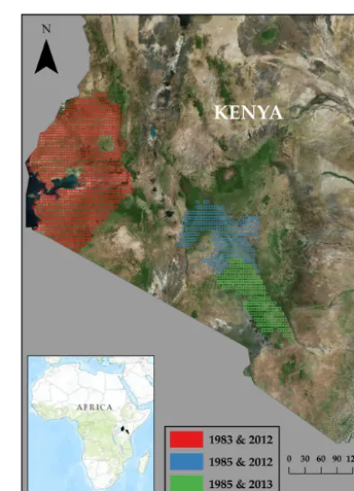
Aerial surveys were conducted in 1983, 1985, 2012, and 2013, to assess changes in land cover over parts of the Lake Victoria basin and central region of Kenya (Machakos and Makueni areas). The surveys yielded 2252 sample area frames of 5 km×5 km covering 28 150 km2 or approxi-mately 47 % of Kenya’s arable lands (Fig. 1). Olofsson et al. (2012) suggest that 5 km×5 km sample area frames are appropriate for evaluating macroscale LULCC models. The lakeshore and lowlands of Lake Victoria basin are primarily tropical, with one long rain season that extends from Febru-ary to September (UNEP, 2008). The neighboring highlands follow a bimodal pattern and annual totals are higher than near the lakeshore, due to warm moist westerlies during the West African monsoon and orographic uplift. Central Kenya is drier and has two distinct rain seasons: long rains (March– June) and short monsoon rains (October–December). The Machakos area, which includes Muranga’, Kiambu, and the
Figure 1.Study area: 1 126 25 km2sample frames demarcating the proportion of land use/cover types estimated from aerial photo in-terpretation and ground surveys. Photos were taken and surveys were performed in western Kenya in 1983 and 2012, north-central Kenya (Machakos area) in 1985 and 2012, and south-central Kenya (Makueni area) in 1985 and 2013. Source of remote sensing im-age and topographic map: Environmental Systems Research Insti-tute (ESRI).
Table 1.Dates on which aerial sample surveys were conducted.
Sample region First survey Second survey Lake Victoria November 1983 October 2012
Machakos March–May 1985 November–December 2012 Makueni June 1985 February 2013
488 m (height above ground) in 1983/1985 and then again in 2012/2013, resulting in approximately seven aerial nat-ural color analogue photos per frame with a ground sam-pling distance of < 1 cm in 1983/1985 and five aerial natural color digital photos per frame with a ground sampling dis-tance of 6.5 cm in 2012/2013. The retrieval dates are shown in Table 1. A team of six technicians interpreted the pho-tos on a rolling basis to minimize potential bias and errors that can occur from manual classification by different inter-preters and for different years. The proportion of each land cover type (0–100 %) was determined by manually classify-ing a grid of 320 randomly distributed points superimposed over each photo. For each year, all land cover types were rep-resented and classified, but not all frames were interpreted and classified (Fig. 1). The interpretations were validated via site visits and meetings with community stakeholders. The estimates were then averaged over the photos across inter-preters to get the proportions for each frame. Further details on the 1983/1985 and 2012/2013 campaigns can be found in EcoSystems Ltd (1983, 1987), and Lamprey (2013).
2.2 Macroscale data handling and processing
The development of the functional relationships from the sample area frames involved four major steps illustrated in Fig. 2. Non-remote-sensing and remote sensing predictors were selected after an exhaustive online search that are freely and seamlessly available across SSA, so that the relationships can be used in future studies across the continent for retro-spective or proretro-spective analyses. Given the large number of predictors collected, machine learning was used to identify a subset of the most powerful predictors before construct-ing the functional relationships. The functional relationships were then evaluated against remote sensing predictors with hold-out samples and finally used to demonstrate how the relationships can be used to reconstruct LULCC estimates continuously through time.
Forty-three non-remote-sensing (climatic, hydrologic, so-cioeconomic, and topographic) and 16 remote sensing (phe-nological) predictors of land cover change were compared and subset for model building with the sample area frames. Either slowly changing (long-term average/one-time value) or dynamic predictors were considered. The slowly chang-ing predictors and their sources are shown in Table 2. Us-ing these predictors alone could streamline the modelUs-ing pro-cess. However, in reality, phenology, climate, and population change frequently, so these predictors were derived on an
an-Figure 2.Model workflow.
nual basis as well. The handling and processing of annually changing or dynamic predictors are discussed in Sect. 2.2.1– 2.2.3. For the remainder of the paper, dynamic predictors in-clude a “.d” extension. All of the geospatial data were pro-jected to Africa Equidistant Conic (m) to facilitate distance calculations. The predictors were resampled to the finest res-olution data (90 m×90 m) and aggregated to 5 km×5 km resolution for model building.
2.2.1 Climate
Bioclimatic (BIOCLIM: Hijmans et al., 2005) variables were used to capture climatic differences in land cover types be-cause they (1) provide biologically meaningful information and (2) have been projected mid-21st century at high spa-tial resolution for SSA (AFRICLIM: Platts et al., 2014). Two additional climate parameters were included in the analysis, because they are potentially relevant and part of the Platts et al. (2014) dataset: atmospheric demand for moisture (poten-tial evapotranspiration – PET) and the moisture index. The BIOCLIM variables were computed on an annual basis from 1983–2012 using monthly temperature, shortwave incoming radiation, and precipitation. The variables were estimated us-ing the “biovars” function in the “dismo” package in R (Hi-jmans et al., 2017). As with the Platts et al. (2014) dataset, PET was estimated using Hargreaves and Samani (1985).
Table 2.Slowly changing (long-term average/one-time value) predictors considered for LULCC estimation and their data sources. Climate, remote sensing, and population predictors were considered as annually changing as well. Dynamic (annual) variables are distinguished with a “.d” extension.
Category Variable Description Units Source
Climate bio1 Annual mean temperature ◦C https://www.york.ac.uk/ environment/research/kite/ resources/
bio2 Mean diurnal range ◦C bio3 Isothermality
bio4 Temperature seasonality ◦C bio5 Maximum temperature of warmest month ◦C bio6 Minimum temperature of coldest month ◦C bio7 Temperature annual range ◦C bio10 Mean temperature of warmest quarter ◦C bio11 Mean temperature of coldest quarter ◦C bio12 Annual precipitation mm bio13 Precipitation of wettest month mm bio14 Precipitation of driest month mm bio15 Precipitation seasonality mm bio16 Precipitation of wettest quarter mm bio17 Precipitation of driest quarter mm mi Moisture index
pet Potential evapotranspiration mm
Hydrology dtw Depth to groundwater mm http://www.bgs.ac.uk/research/ groundwater/international/ africanGroundwater/maps.html gwp Groundwater productivity L s−1
gws Groundwater storage mm
Phenological ampl Linear amplitude https://ecocast.arc.nasa.gov/data/ pub/gimms/
ampn Nonlinear amplitude
lint Linear intercept (annual mean) nint Nonlinear intercept (annual mean) phsl Linear phase
phsn Nonlinear phase
strn Nonlinear strength (asymmetry) warpn Nonlinear warp (asymmetry)
Socioeconomic popd Population density no. of people km−2 http://na.unep.net/siouxfalls/ datasets/datalist.php
Topography asp Aspect ◦ http://www.cgiar-csi.org/data/srtm-90m-digital-elevation
elev Elevation m
slp Slope %
topind Topographic wetness index
time step and 0.1◦ (∼10 km×10 km at the Equator) reso-lution. CHIRPS is available at pentad (5-day) intervals and 0.05◦(∼5 km×5 km at the Equator) spatial resolution from 1981 to 2012. Like PHF, CHIRPS is a blend of several observation-based, remote sensing, and reanalysis sources: geostationary thermal infrared satellite observations from the Climate Prediction Center and National Climatic Data Cen-ter, TRMM, and NOAA-NCAR. CHIRPS was selected as the
2.2.2 Population density
Population density was derived from the UNEP/GRID-Sioux Falls African Population Distribution Database (APDD) on an annual basis from 1983 to 2012. APDD consists of population density at a spatial resolution of 2.5 arcmin (∼5 km×5 km at the Equator) for base years 1960, 1970, 1980, 1990, and 2000. The grids are derived from popu-lation statistics at various administrative (district, province, etc.) levels and temporal scales, depending on the avail-ability of national population statistics. A detailed descrip-tion of the derivadescrip-tion of gridded populadescrip-tion can be found in Deichmann (1996). Each grid cell represents “popula-tion potential”, based on its proximity to the transporta-tion network (roads, railroads, and navigable rivers, and ma-jor towns/cities). Population at a given administrative level is then disaggregated according to the population potential. Grid cells that are closer to the network have higher coeffi-cients and therefore receive a larger proportion of the popula-tion than grid cells further away. The base years are then ex-trapolated with an exponential growth/decay function (Davis, 1995). For consistency, the same function was used to dis-tribute population between base years on an annual basis for each grid cell:
Pi,j,t=Pi,j,Te1t ki,j, (1)
ki,j =ln PT+10n/PT+10(n−1)/10. (2)
Pi,j,t is the interpolated population/population density for a given year (t) and at grid cell i, j; Pi,j,T is the population/population density for a given base year (pe-riod=10 years); 1t is the change in time from the base year to the year being interpolated; and ki,j (Eq. 2) is the growth/decay coefficient. The growth/decay coefficient is de-fined by PT+10(n−1) (initial base year for iteration n) and PT+10n(last base year for iterationn). The denominator was set to 10, because ki,j accounted for decadal trends. After 2000, population statistics were extrapolated to 2012 using the 1990–2000 growth/decay coefficients.
2.2.3 Remote sensing predictors
The National Aeronautics and Space Administration’s Global Inventory Modeling and Mapping Studies (GIMMS) normalized difference vegetation index (NDVI) version 3 (NDVI3g) (Pinzon and Tucker, 2014) was used to estimate the remote sensing predictors. NDVI is a ratio-based vegeta-tion index derived from Earth observavegeta-tion (AVHRR) surface reflectance in the visible red and near infrared (NIR). NDVI approaching one (zero) is indicative of dense vegetation (bare soil). NDVI3g is available at 0.08◦ (∼8 km×8 km at the Equator) spatial resolution and at a 15-day time step from 1983 to 2013. NDVI3g has been compared to other long-term global vegetation records and is considered the most appropriate for trend analyses (Tian et al., 2015).
The predictors were derived from NDVI using harmonic regression (Eastman et al., 2009) on an annual basis from 1983 to 2012. Linear harmonic regression estimates the am-plitude (maximum) and phase (timing) of a fitted time se-ries, but unless higher-order harmonics are introduced, linear harmonic regression is too rigid to account for outliers and multimodal regimes commonly found in the tropics. To over-come these obstacles, nonlinear harmonic regression (Carrão et al., 2010) was used to estimate five phenological predic-tors:
NDVIi,j,T=Mi,j+Ai,jcos (ω0t+∅+αcos (ω0t+ϕ)), (3)
where NDVIi,j,T is NDVI at grid celli,j and over period
T, which in this case was 24, because nonlinear harmonic regression was computed on an annual basis from the 15-day data;M is the intercept (annual mean NDVI);Ais the amplitude;φ is the annual phase; andα andϕ are nonlin-ear terms defining the strength of nonlinnonlin-earity (asymmetry) and nonlinear phase (deceleration/acceleration of asymme-try), respectively. The frequency (ω0) equals 2π/T. The ap-proach can be reduced to a linear harmonic oscillator by set-ting αcos(ω0t+ϕ) to zero. The nonlinear predictors were derived at each grid cell using the “nlsLM” function in the “minipack.lm” package in R (Elzhov et al., 2016). The nl-sLM function uses the Levenberg–Marquardt optimization method (Moré, 1978) to find the nonlinear least-squares fit. The function was constrained by the seed and boundary con-ditions described in Carrão et al. (2010). One thousand iter-ations at each grid cell were performed to avoid fitting local optima. Linear terms (Aandφ) were computed for the anal-ysis as well, using the “lm” function in the “stats” package in R (https://cran.r-project.org/), because they are more effi-cient and are easier to interpret.
2.3 Land cover model development using remote sensing and non-remote-sensing predictors
Land cover models were developed for each level of speci-ficity. Seventy percent of the samples (N=1576) were used for model calibration and 30 % of the samples (N=676) were used for model validation.
and independent decision trees consisting of various combi-nations of predictors and sample subsets. The performance of the ensemble was measured with a pseudo-coefficient of determination (pseudo-R2), which is one minus the ratio of the cross-validated mean squared error (MSE) of the predic-tion to the variance of the observed data. As MSE or the average error between predicted and observed estimates ap-proaches zero,R2approaches one (perfect correlation). The importance of each predictor in the ensemble is also quanti-fied and is defined by the percent increase in cross-validated MSE when a predictor is removed from the ensemble. Once the predictors were ranked, the “rfcv” function was used to determine the number of predictors to use to develop tional relationships for each land cover class. The rfcv func-tion computes the cross-validated MSE versus the number of predictors included in the ensemble in descending order of importance.
The drawback of RF is that it results in complex rela-tionships that are difficult to interpret. Generalized additive models (GAMs) (Hastie and Tibshirani, 1990) were used to build functional relationships on the subsets of important predictors identified with RF because a number of studies have successfully estimated the proportion of crop area with socio-ecological predictors and GAMs (Grace et al., 2014; Husak et al., 2008; Marshall et al., 2011); like RF, GAMs are not severely impacted by nonlinear data, and unlike RF, GAMs are relatively simple and easy to interpret. Since the response variable (proportion of land cover type) was contin-uous and bounded from 0 to 100 %, the data were fitted us-ing a quasi-binomial distribution (link: logistic). The logistic GAM predicts the log likelihood of an event (probability of success/probability of failure) using, in our case, a series of cubic spline functions:
log
p
j
1−pj
=β0+ X
fi,j xi,j, (4)
wherepis the probability of a LULC type for sample area framej,β0is the intercept, andfi,j (xi,j) is the cubic spline function for predictorxi at sample area framej. The GAMs were developed with the “gam” function in the “mgcv” pack-age in R. Model calibration was evaluated with explained part and overall deviance. Deviance is the log likelihood (probability space) alternative to variance. Part deviance is the deviance explained when the target predictor is removed from a GAM minus the overall deviance. Another pseudo-R2 statistic (1−model deviance/null deviance) was also com-puted to compare calibration with validation.
In order to demonstrate how the models can be used for macroscale application, the final GAMs developed were em-ployed to reconstruct the annual change in agriculture and natural vegetation and to perform a trend analysis from 1983 to 2012 at each sample area frame. Trends were estimated using the Theil–Sen technique, which computes the median of all possible pairwise slopes in a time series. The approach has been used, for example, to measure long-term trends in
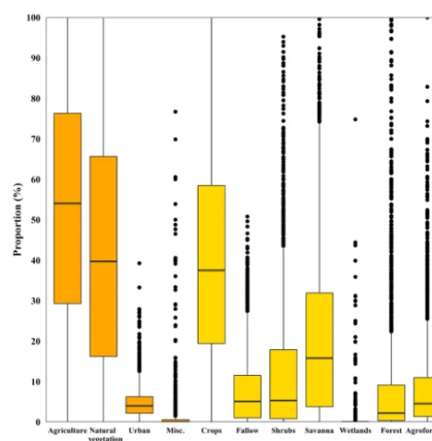
Figure 3.Box plot of the proportion of land cover types for two levels of classification (N=2252). The first and second levels of classification are shaded in orange and yellow, respectively.
NDVI (de Beurs and Henebry, 2005), because it is not signif-icantly impacted by outliers or nonlinearity. The significance of each trend was assessed using the Mann–Kendall statistic. Trends were masked at the 99.9 % confidence band.
3 Results
3.1 Land cover sample area frame summary
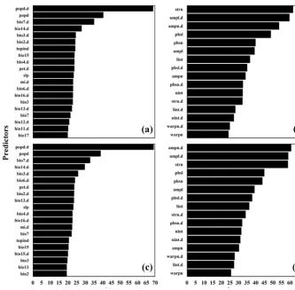
Figure 4.Percent mean squared error (MSE) increase after each of the top 20 non-remote-sensing(a, c)and 16 remote sensing(b, d) predic-tors were omitted from the random forest ensemble model predicting the proportion of agriculture and natural vegetation in the calibration sample frames, respectively. The models explained 69, 49, 69, and 50 % of the proportion variability.
smallest proportion of land cover (median=2.22 %) but had a large number of outliers.
3.2 Data reduction
The top remote sensing and non-remote-sensing predic-tors considered are ranked in descending order of impor-tance for agriculture and natural vegetation using bar graphs in Fig. 4. The RF ensemble models using non-remote-sensing predictors performed moderately well for agricul-ture (pseudo-R2=0.69) and natural vegetation (pseudo-R2=0.69) but poorly for the more nonlinear distribu-tions (urban pseudo-R2=0.37 and miscellaneous pseudo-R2=0.50). The RF ensemble models using remote sens-ing predictors all performed poorly: agriculture (pseudo-R2=0.49), natural vegetation (pseudo-R2=0.50), urban (pseudo-R2=0.22), and miscellaneous (pseudo-R2=0.33). It should be noted in each case, however, that the highest-ranked remote sensing predictors resulted in lower model er-ror than the highest-ranked non-remote-sensing predictors. The non-remote-sensing predictors were more numerous and generated larger incremental improvements that contributed
to overall greater predictive power. For the non-remote-sensing ensembles, dynamic predictors were more impor-tant than slowly changing predictors, and population density and climate predictors consistently outranked topographic or hydrologic predictors. Popd.d, popd, bio7.d, bio14.d, and bio3.d were consistently ranked the most important predic-tors of agriculture and natural vegetation proportions. Omit-ting popd.d, the most important predictor for agriculture, for example, led to a more than 65 % increase in ensem-ble MSE. Given that popd.d and popd were both important, model results were compared with popd.d and popd individ-ually and combined as anomalies (popd.d/popd). Ensemble performance was better when the two predictors were con-sidered separately. The most important remote sensing pre-dictors were less influential than popd.d; strn, ampn.d, and ampl.d were more equally important for agriculture and nat-ural vegetation, followed by phsl and phsn.
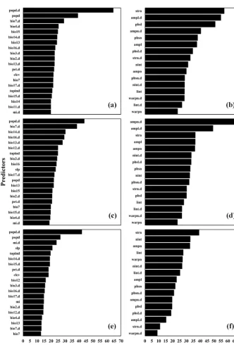
variabil-Figure 5.Percent mean squared error (MSE) increase after each of the top 20 non-remote-sensing(a, c, e)and 16 remote sensing(b, d, f) pre-dictors were omitted from the random forest ensemble model predicting the proportion of crops, savanna, and forest in the calibration sample frames, respectively. The models explained 63, 46, 62, 44, 62, and 46 % of the proportion variability.
ity than the level one RF ensemble models and the non-remote-sensing predictors outperformed the remote sens-ing predictors when more than the highest-ranked predic-tors were introduced. The non-remote-sensing models per-formed moderately well for crops (pseudo-R2=0.63), sa-vanna (pseudo-R2=0.62), and forest (pseudo-R2=0.61) but poorly for fallow (pseudo-R2=0.42), shrubs (pseudo-R2=0.54), wetlands (pseudo-R2=0.10), and agroforestry (pseudo-R2=0.55). Precipitation-based climatic predictors
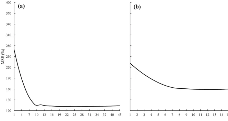
(pseudo-Figure 6.Curves showing the mean squared error (MSE) of the predicted proportion of forest from the random forest ensembles parameter-ized with non-remote-sensing(a)and remote sensing (b)predictors. The number of predictors corresponds to the bar graphs in descending order of importance.
R2=0.46), and agroforestry (pseudo-R2=0.41). For crops, strn and ampl.d remained the most important predictors. Maximum annual NDVI, as captured by ampl.d and ampn.d, was much more important for predicting the proportion of savanna. Unlike other ensembles, which were driven by dy-namic predictors, the most important remote sensing predic-tors for forest cover were long-term averages.
3.3 Building functional relationships
The GAMs were developed for moderately performing land cover classes and used considerably fewer predictors than the RF ensembles, because most of the predictors in the ensem-bles explained very little, if any, variance. This is illustrated in Fig. 6, which shows MSE versus the number of predic-tors used in the non-remote-sensing and remote sensing en-sembles for forest cover. For the non-remote-sensing ensem-ble, MSE increased from 119.76 to 120.49 after the 10th predictor and leveled off after the 13th predictor were in-troduced. For the remote sensing ensemble, MSE increased from 120.49 to 163.34 and leveled off after the 7th predictor was introduced. For this reason, the GAMs were built with 10–13 of the highest-ranked non-remote-sensing predictors and additional predictors, namely popd, were removed after redundancies were identified in the GAM component func-tional plots and with significance tests (not shown). GAMs were not constructed using the remote sensing predictors be-cause of the poor results of the ensembles and the inability of additional predictors to substantially improve the accuracy of the GAMs. Similarly, non-remote-sensing GAMs were not developed for urban, miscellaneous, fallow, shrubs, or wet-lands.
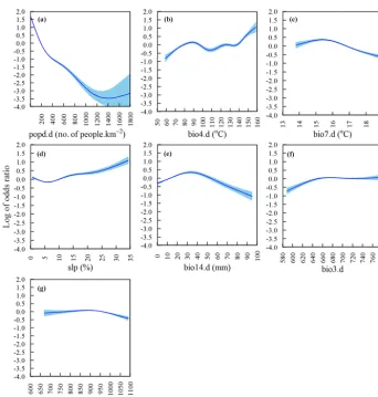
Figure 7.Partial functional plots relating the proportion (probability) of agriculture expressed as the log of odds ratio with(a)population density (popd.d),(b)precipitation of driest month (bio14.d),(c)topographic wetness index (topind),(d)mean diurnal range (bio2.d),(e) pre-cipitation seasonality (bio15),(f)temperature seasonality (bio4.d),(g)slope (slp),(h)moisture index (mi.d), and isothermality (bio3.d). The probabilities are defined using a logistic model with cubic smoothing splines (N=1,576).
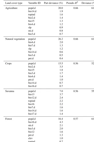
which is the difference between the annual maximum and minimum temperatures. Areas that are less isothermal es-sentially have more pronounced seasons and are climatically less tropical. For the level two classifications, calibration was more difficult and yielded poorer relationships. Popd.d was the most important predictor and explained 7.0–16.4 % unique deviance. The predictive power of the topographic and climatic variables was more equally distributed than for the level one classification.
In all cases, the R2 for the validation subset was lower than the pseudo-R2 from the calibration subset: agricul-ture (1R2= −0.04), natural vegetation (1R2= −0.01), crops (1R2= −0.03), savanna (1R2= −0.01), and forest (1R2= −0.06) (Fig. 9). With the exception of the crops GAM, level two GAMs tended to under-predict high propor-tions of land cover (savanna and forest) and contained nu-merous outliers.
3.4 Trend analysis
Table 3.Calibration statistics of the generalized additive models used to predict the proportion of land cover (N=1576). Predictors are significant at the 99.9 % confidence band.
Land cover type Variable ID Part deviance (%) Pseudo-R2 Deviance (%)
Agriculture popd.d 20.0 0.66 61.5
bio14.d 1.9
topind 1.6
bio2.d 1.4
bio15 1.3
bio4.d 1.2
slp 0.9
mi.d 0.8
bio3.d 0.7
Natural vegetation popd.d 26.2 0.66 61.4
bio4.d 2.0
bio7.d 1.3
slp 1.2
bio14.d 0.6
bio3.d 0.5
pet.d 0.4
Crops popd.d 15.5 0.56 52.1
bio2.d 3.5
bio15 1.8
bio3.d 1.7
bio4.d 1.4
pet.d 1.0
bio14.d 0.7
bio16.d 0.7
Savanna popd.d 7.0 0.56 55.7
bio13 3.7
bio12.d 2.4
topind 2.2
bio16 2.2
bio7.d 1.6
bio14.d 1.6
bio17.d 1.4
Forest popd.d 16.4 0.57 61.2
bio16.d 4.3
mi.d 2.1
bio3.d 2.0
bio12 1.6
pet.d 1.3
elev 1.0
topind 0.7
bio14.d 0.7
slp 0.7
and high-potential agricultural zones of central Kenya. The only decrease in agricultural lands was in the town of Kitale (−1.40 % per year). The time series is also shown in Fig. 10d. Population density in Kitale was 1110 people km−2in 1983, which is near the threshold of declining agriculture cover versus population density at 1200 people km−2. By 2009, when the largest decrease in agriculture cover occurred, from
Figure 8.Partial functional plots relating the proportion (probability) of natural vegetation expressed as the log of odds ratio with(a) pop-ulation density (popd.d),(b)temperature, seasonality (bio4.d),(c)temperature annual range (bio7.d),(d)slope (slp),(e)precipitation of the driest month (bio14.d),(f)isothermality (bio3.d), and(g)potential evapotranspiration (pet.d). The probabilities are defined using a logistic model with cubic smoothing splines (N=1576).
4 Discussion
The results make three important contributions that the land surface modeling community should consider to improve LULCC detection, particularly for SSA: (1) a socioeconomic variable (population density) was the highest-ranked predic-tor of LULCC and had considerably more predictive power than biophysical predictors, (2) non-remote-sensing predic-tors outperformed remote sensing predicpredic-tors due to their number and the incremental improvement in the predictive power of each, and (3) coarse-resolution data were able to capture general classification descriptors, but unable to cap-ture more detailed descriptors.
The global increase in agricultural land cover has been at-tributed to the demand for food and other agricultural com-modities by a growing population (Pongratz et al., 2008). In SSA, smallholder farms, which support the majority of the labor force, are small (half are < 1.5 ha) and concen-trated in densely populated areas, while large portions of
Figure 9.Predicted versus observed proportion of agriculture(a); natural vegetation(b); crops(c); savanna(d); and forest(e)for the validation subset (N=676). The 1:1 line is drawn through the ori-gin.
1200 people km−2, as in Kitale, so it is difficult to know whether this functional relationship holds for very high popu-lation densities. At least to 2008, Kitale experienced a growth rate of 12 %, well above the national average (7 %), due to persistent drought and out-migration from neighboring high-production zones (Majale, 2008). Although the functional re-lationship for population density corroborates household sur-veys in Kenya and other agrarian countries in SSA, it should be further scrutinized, because land tenure in SSA is com-plex (Place, 2009), the dependency of LULCC predictors on location and spatial scale can be high (Rindfuss et al., 2004), and the transition from agrarian to industrialized nations may make 50–100-year projections for SSA obsolete.
The proposed methodology when applied to other regions of the world will undoubtedly result in a different combina-tion of socio-ecological predictors and funccombina-tional relacombina-tion- relation-ships, because access to land varies across agrarian and non-agrarian societies, so further study is required with observed data to develop region-specific models and validate the re-sults for countries in SSA. Kumar et al. (2013), for example, showed that in the United States pre-1900, when the country
was largely agrarian and transportation networks were weak, population density and crop area were directly correlated, be-cause crops needed to be grown close to markets. However, as the country became more industrialized and transporta-tion networks improved, farmers moved to more biophysi-cally suitable areas away from city centers, making biophys-ical determinants of crop area more important than popula-tion density in the latter half of the 20th century. Whether the analyses are performed in agrarian or non-agrarian regions, extensive preparation of observation data will be required, because the data used in this study, namely consistent sample area frames at a spatial resolution appropriate for land sur-face modeling and spanning multiple climatic zones through time, are quite unique.
Population density estimates vary widely (Wilson, 2014), and given its fundamental importance to the proposed model framework, future work should aim to integrate a more dy-namic product that better accounts for interannual variability and realistic representation of current and projected popu-lation density. To the authors’ knowledge, this was the first attempt to make a population product dynamic. However, the approach is essentially tracking decadal trends that ex-plain a significant portion of interannual variability. In real-ity, population density can show high interannual variability due to migration and other factors. Regarding the product it-self, changes in population density do not necessarily “grow” from transportation networks and are influenced by impor-tant feedbacks now and in the future. In addition, the extrap-olation method used is efficient and can be projected indefi-nitely, but does not capture complex demographics that other methods do and can lead to “runaway” growth/decline and unrealistic mid- to late-21st century projections for scenario-building (Baker et al., 2008). Finally, there is no consensus on which population product to use however, in the future, other products (e.g., Afripop) should be compared against the product used here, used to adjust growth/decay coefficient for population density estimates beyond 2000, or combined to make a model ensemble.
avail-Figure 10.Simulated percent agriculture for sample area frames in 1983(a)and 2012(b), change in agriculture per year over the 30 year (1983–2012) period(c), and time series of the strongest positive (red) and negative (blue) trend(d). Trends were determined with a Theil–Sen estimator and masked for significance using the Man–Kendall statistic at the 99.9 % confidence band.
able mid- and late 21st century and are therefore widely used for prospective analyses, so methods should be explored to project soils and socio-economic data into the future to im-prove LULCC estimates.
Grace et al. (2014) developed GAMs to predict cropped area in Kenya using biophysical predictors (rainfall, ele-vation, NDVI, slope, and the topographic wetness index) and explained much of the deviance in cropped area (41.9– 81.4 %). Although the models used different predictors for different years and production zones, and the definition of cropped area and the degree of functional smoothing were not explicit, the study shows that the intercorrelation among predictors may be obscuring the importance of biophysi-cal determinants. Specifibiophysi-cally, population density tends to be highly correlated with and could be suppressing the ex-planatory power of biophysical predictors, though the partial deviance statistics did not reflect this. In addition, the ran-dom forest algorithm accounts for intercorrelation to some degree, but other techniques could be introduced to further reduce these effects. For example, principal component
captured using coarse-resolution data, because this predic-tor changes more gradually over space. An analysis of the non-remote-sensing and remote sensing predictors together revealed that for agriculture, natural vegetation, savanna, and forest cover, Earth observation data provided an additional 1–2 % explained deviance. If the long-term average remote sensing predictors could be downscaled using MODIS or Landsat data and then aggregated to 5 km×5 km resolution with distribution moments as predictors, for example, the ex-planatory power of non-remote-sensing predictors could be further enhanced for retrospective analyses. Another avenue worth exploring could involve using downscaled long-term average remote sensing predictors to develop 5 km×5 km probabilities as in the Pengra et al. (2015) dataset to evaluate the non-remote-sensing models proposed here.
The evaluation of the models at two levels of specificity revealed that coarse resolution is able to better simulate gen-eral descriptors, such as natural vegetation, but is poorer at predicting more detailed descriptors, such as forest. Each of the more detailed random forest ensembles with non-remote-sensing predictors had 1R2s of −0.06, −0.07, and −0.07 for crop, savanna, and forest over agriculture and natural vegetation, respectively. Part of this discrepancy can be at-tributed to the increased interpretation uncertainty, as inter-preters find it more challenging to distinguish between more detailed LULC types. In addition, coarse-resolution data may not be able to capture the level of heterogeneity in the area sample frames needed to distinguish land-use/cover-specific socio-ecological patterns and properties.
5 Conclusion
This study developed and evaluated a simple method to pro-vide consistent estimates of LULCC annually over 30 years at 5 km×5 km resolution using non-parametric functional relationships with a small subset of socio-ecological predic-tors (p≤10). Functional relationships were developed after data-mining 43 geospatial datasets that are available seam-lessly across SSA, which can be used for retrospective or prospective mid- and late-21st century analyses as well. The relationships are intuitive and tunable, making their use prac-tical for decision makers to identify intervention hotspots and develop land management scenarios. Model validation, performed with the proportion of major land cover types in Kenya over a 30-year period, revealed that a number of activ-ities should be performed to improve the predictive power of the models for practical use. These activities should include integrating improved existing or newly developed spatially explicit geospatial (particularly socioeconomic) datasets into the proposed model framework. With these improvements, land surface and LULCC modeling could be greatly en-hanced and the consequence of the latter on the Earth system more fully understood. In an upcoming study, the modeling approach proposed here will be used with a newly acquired
sample area frame dataset to estimate historical LULCC and project land suitability across SSA mid-21st century with AFRICLIM and population statistics.
6 Data availability
All input geospatial data, sample area frame proportions of land use/cover, and model outputs will be made freely avail-able on the World Agroforestry Centre’s Landscapes Portal (http://landscapeportal.org/). Other data used in this study not on the Landscapes portal, including AFRICLIM (Platts et al., 2014), quantitative groundwater maps for Africa (MacDonald et al., 2012), GIMMMS NDVI3g (Pinzon and Tucker, 2014), UNEP/GRID, 1987, CGIAR-CSI SRTM 90m (Jarvis et al., 2008), CHIRPS (Funk et al, 2014), and PHF (Chaney et al., 2014), are available at https://www.york.ac. uk/environment/research/kite/resources/; http://www.bgs.ac. uk/research/groundwater/international/africanGroundwater/ maps.html; https://ecocast.arc.nasa.gov/data/pub/gimms/; http://na.unep.net/siouxfalls/datasets/datalist.php;
http://www.cgiar-csi.org/data/srtm-90m-digital-elevation; http://chg.geog.ucsb.edu/data/; and http://hydrology. princeton.edu/data.php.
Competing interests. The authors declare that they have no con-flict of interest.
Acknowledgements. The work summarized in this manuscript was primarily funded through support by the CGIAR Research Program on Climate Change, Agriculture and Food Security for the project titled “Multi-disciplinary species distribution mod-elling for “climate smart” agriculture in East Africa”. Additional support for the early field and aerial surveys was supported by the Kenyan Lake Basin Development Authority and Ministry of Planning and National Development. We would like to extend our special thanks to Sandra Nakibilango, Dorcas Ninsiima, Charles Ngugi, Patrick Ojorot, and Samuel Olowo, who inter-preted the aerial photos taken for this project; Bernadette Apio, who coordinated the interpreter team; and Juliet Kyakobyewo, who entered the data into our database. Finally, we would like to thank Eike Luedeling, who initially led and organized the project.
Edited by: Z. Xie
Reviewed by: five anonymous referees
References
Alcamo, J., Schaldach, R., Koch, J., Kölking, C., Lapola, D., and Priess, J.: Evaluation of an integrated land use change model in-cluding a scenario analysis of land use change for continental Africa, Environ. Model. Softw., 26, 1017–1027, 2011.
Anderson-Teixeira, K. J. and DeLucia, E. H.: The greenhouse gas value of ecosystems, Glob. Change Biol., 17, 425–438, 2011. Baker, J., Ruan, X., Alcantara, A., Jones, T., Watkins, K.,
Mc-Daniel, M., Frey, M., Crouse, N., Rajbhandari, R., Morehouse, J., Sanchez, J., Inglis, M., Baros, S., Penman, S., Morrison, S., Budge, T., and Stallcup, W.: Density-dependence in urban hous-ing unit growth: An evaluation of the Pearl-Reed model for pre-dicting housing unit stock at the census tract level, J. Econ. Soc. Meas. 33, 155–163, 2008.
Ban, Y., Gong, P., and Giri, C.: Global land cover mapping us-ing Earth observation satellite data: Recent progresses and chal-lenges, ISPRS J. Photogramm., 103, 1–6, 2015.
Binder, H. and Tutz, G.: A comparison of methods for the fitting of generalized additive models, Stat. Comput., 18, 87–99, 2007. Breiman, L.: Random Forests, Mach. Learn., 45, 5–32, 2001. Carrão, H., Gonalves, P., and Caetano, M.: A Nonlinear Harmonic
Model for Fitting Satellite Image Time Series: Analysis and Pre-diction of Land Cover Dynamics, IEEE T. Geosci. Remote, 48, 1919–1930, 2010.
Chaney, N. W., Sheffield, J., Villarini, G., and Wood, E. F.: Development of a High-Resolution Gridded Daily Meteoro-logical Dataset over Sub-Saharan Africa: Spatial Analysis of Trends in Climate Extremes, J. Climate, 27, 5815–5835, doi:10.1175/JCLI-D-13-00423.1, 2014 (data available at: http:// hydrology.princeton.edu/data.php, last access: 18 August 2016). Chen, J., Chen, J., Liao, A., Cao, X., Chen, L., Chen, X., He, C., Han, G., Peng, S., Lu, M., Zhang, W., Tong, X., and Mills, J.: Global land cover mapping at 30 m resolution: A POK-based op-erational approach, ISPRS J. Photogramm., 103, 7–27, 2015. Davin, E. L. and de Noblet-Ducoudré, N.: Climatic Impact of
Global-Scale Deforestation: Radiative versus Nonradiative Pro-cesses, J. Climate, 23, 97–112, 2010.
Davis, H. C.: Demographic Projection Techniques for Regions and Smaller Areas: A Primer, UBC Press, Vancouver, Canada, UBC Press, 116 pp., 1995.
de Beurs, K. M. and Henebry, G. M.: A statistical framework for the analysis of long image time series, Int. J. Remote Sens., 26, 1551–1573, 2005.
de Bie, C. A. J. M., Nguyen, T. T. H., Ali, A., Scarrott, R., and Skidmore, A. K.: LaHMa: a landscape heterogeneity mapping method using hyper-temporal datasets, Int. J. Geogr. Inf. Sci., 26, 2177–2192, 2012.
DeFries, R. S., Field, C. B., Fung, I., Justice, C. O., Los, S., Mat-son, P. A., Matthews, E., Mooney, H. A., Potter, C. S., Prentice, K., Sellers, P. J., Townshend, J. R. G., Tucker, C. J., Ustin, S. L., and Vitousek, P. M.: Mapping the land surface for global atmosphere-biosphere models: Toward continuous distributions of vegetation’s functional properties, J. Geophys. Res.-Atmos., 100, 20867–20882, 1995.
Deichmann, U.: A Review of Spatial Population Database Design and Modeling (Technical Report No. 96-3), National Center for Geographic Information and Analysis, Santa Barbara, CA, 1996. Eastman, R., Sangermano, F., Ghimire, B., Zhu, H., Chen, H., Neeti, N., Cai, Y., Machado, E. A., and Crema, S. C.: Seasonal trend analysis of image time series, Int. J. Remote Sens., 30, 2721– 2726, doi:10.1080/01431160902755338, 2009.
EcoSystems Ltd: Integrated Land Use Survey: Final Report. Lake Basin Development Authority, Kisumu, Kenya, 1983.
EcoSystems Ltd: Integrated Land Use Database for Kenya. Minstry of Planning & Natural Development, Nairobi, Kenya, 1987. Elzhov, T. V., Mullen, K. M., Spiess, A. N., and Bolker, B.: R
In-terface to the Levenberg-Marquardt Nonlinear Least-Squares Al-gorithm Found in MINPACK, Plus Support for Bounds, 14 pp., Repository, CRAN, 2016.
Fernández-Delgado, M., Cernadas, E., Barro, S., and Amorim, D.: Do We Need Hundreds of Classifiers to Solve Real World Clas-sification Problems? J. Mach. Learn. Res., 15, 3133–3181, 2014. Funk, C., Peterson, P., Landsfeld, M., Pedreros, D., Verdin, J., Row-land, J., Romero, B., Husak, G. J., Michaelsen, J., and Verdin, A.: A Quasi-Global Precipitation Time Series for Drought Monitor-ing (No. 832), US Geological Survey Data Series, US Geological Survey, Washington, DC, available at: http://chg.geog.ucsb.edu/ data/ (last access: 15 Feburary 2015), 2014.
Funk, C., Verdin, A., Michaelsen, J., Peterson, P., Pedreros, D., and Husak, G.: A global satellite-assisted precipitation climatology, Earth Syst. Sci. Data, 7, 275–287, doi:10.5194/essd-7-275-2015, 2015.
Giri, C., Pengra, B., Long, J., and Loveland, T. R.: Next generation of global land cover characterization, mapping, and monitoring, Int. J. Appl. Earth Obs., 25, 30–37, 2013.
Grace, K., Husak, G., and Bogle, S.: Estimating agricultural pro-duction in marginal and food insecure areas in Kenya using very high resolution remotely sensed imagery, Appl. Geogr., 55, 257– 265, 2014.
Hansen, M. C., Stehman, S. V., and Potapov, P. V.: Quantification of global gross forest cover loss, P. Natl. Acad. Sci. USA, 107, 8650–8655, 2010.
Hansen, M. C. and Loveland, T. R.: A review of large area mon-itoring of land cover change using Landsat data, Remote Sens. Environ., Landsat Legacy Special Issue, 122, 66–74, 2012. Hargreaves, G. H. and Samani, Z. A.: Reference Crop
Evapotran-spiration from Temperature, Appl. Eng. Agric., 1, 96–99, 1985. Hastie, T. J. and Tibshirani, R. J.: Generalized Additive Models,
CRC Press, Chapman and Hall/CRC Boca Raton, Florida, USA, 353 pp., 1990.
Held, I. M. and Soden, B. J.: Robust Responses of the Hydrological Cycle to Global Warming, J. Climate, 19, 5686–5699, 2006. Heistermann, M., Müller, C., and Ronneberger, K.: Land in sight?:
Achievements, deficits and potentials of continental to global scale land-use modeling, Agric. Ecosyst. Environ., 114, 141– 158, 2006.
Hijmans, R. J., Cameron, S. E., Parra, J. L., Jones, P. G., and Jarvis, A.: Very high resolution interpolated climate surfaces for global land areas, Int. J. Climatol., 25, 1965–1978, 2005.
Hijmans, R. J., Phillips, S., Leathwick, J., and Elith, J.: Species Dis-tribution Modeling, 68 pp., Repository, CRAN, 9 January 2017. Husak, G. J., Marshall, M. T., Michaelsen, J., Pedreros, D.,
Funk, C., and Galu, G.: Crop area estimation using high and medium resolution satellite imagery in areas with com-plex topography, J. Geophys. Res.-Atmos., 113, D14112, doi:10.1029/2007JD009175, 2008.
Jayne, T. S. and Muyanga, M.: Land constraints in Kenya’s densely populated rural areas: implications for food policy and institu-tional reform, Food Secur., 4, 399–421, 2012.
Jayne, T. S., Yamano, T., Weber, M. T., Tschirley, D., Benfica, R., Chapoto, A., and Zulu, B.: Smallholder income and land distri-bution in Africa: implications for poverty reduction strategies, Food Policy, 28, 253–275, 2003.
Kumar, S., Merwade, V., Rao, P. S. C., and Pijanowski, B. C.: Char-acterizing Long-Term Land Use/Cover Change in the United States from 1850–2000 Using a Nonlinear Bi-analytical Model, Ambio, 42, 285–297, 2013.
Lambin, E. F., Geist, H. J., and Lepers, E.: Dynamics of Land-Use and Land-Cover Change in Tropical Regions, Annu. Rev. Envi-ron. Resour., 28, 205–241, 2003.
Lamprey, R. H.: Aerial Point Sampling (APS) Survey: Lake Basin, Machakos and Makueni, Kenya, 2012–13, Nairobi, Kenya, 2013. Lawrence, P. J., Feddema, J. J., Bonan, G. B., Meehl, G. A., O’Neill, B. C., Oleson, K. W., Levis, S., Lawrence, D. M., Kluzek, E., Lindsay, K., and Thornton, P. E.: Simulating the Biogeochemi-cal and BiogeophysiBiogeochemi-cal Impacts of Transient Land Cover Change and Wood Harvest in the Community Climate System Model (CCSM4) from 1850 to 2100, J. Climate, 25, 3071–3095, 2012. Lepers, E., Lambin, E. F., Janetos, A. C., DeFries, R., Achard, F.,
Ramankutty, N., and Scholes, R. J.: A Synthesis of Information on Rapid Land-cover Change for the Period 1981–2000, Bio-Science, 55, 115–124, 2005.
MacDonald, A. M., Bonsor, H. C., Dochartaigh, B. É. Ó., and Tay-lor, R. G.: Quantitative maps of groundwater resources in Africa, Environ. Res. Lett., 7, 1–7, doi:10.1088/1748-9326/7/2/024009, 2012 (data available at: http://www.bgs.ac.uk/research/ groundwater/international/africanGroundwater/maps.html, last access: 23 July 2015).
Majale, M.: Employment creation through participatory urban plan-ning and slum upgrading: The case of Kitale, Kenya. Habitat Int., Labour in Urban Areas, 32, 270–282, 2008.
Makarieva, A. M., Gorshkov, V. G., and Li, B.-L.: Revisiting forest impact on atmospheric water vapor transport and precipitation, Theor. Appl. Climatol., 111, 79–96, 2013.
Marshall, M. T., Husak, G. J., Michaelsen, J., Funk, C., Pe-dreros, D., and Adoum, A.: Testing a high-resolution satel-lite interpretation technique for crop area monitoring in de-veloping countries, Int. J. Remote Sens., 32, 7997–8012, doi:10.1080/01431161.2010.532168, 2011.
Meiyappan, P., Dalton, M., O’Neill, B. C., and Jain, A. K.: Spatial modeling of agricultural land use change at global scale, Ecol. Model., 291, 152–174, 2014.
Moré, J. J.: The Levenberg-Marquardt algorithm: Implementation and theory, in: Numerical Analysis, Lecture Notes in Mathemat-ics, edited by: Watson, G. A., Springer Berlin Heidelberg, 105– 116, 1978.
Ngetich, K. F., Mucheru-Muna, M., Mugwe, J. N., Shisanya, C. A., Diels, J., and Mugendi, D. N.: Length of growing season, rainfall temporal distribution, onset and cessation dates in the Kenyan highlands, Agric. For. Meteorol., 188, 24–32, 2014.
Norton-Griffiths, M.: Aerial Point Sampling for Land Use Surveys, J. Biogeogr., 15, 149–156, 1988.
Olofsson, P., Stehman, S. V., Woodcock, C. E., Sulla-Menashe, D., Sibley, A. M., Newell, J. D., Friedl, M. A., and Herold, M.: A
global land-cover validation data set, part I: fundamental design principles, Int. J. Remote Sens., 33, 5768–5788, 2012.
Pengra, B., Long, J., Dahal, D., Stehman, S. V., and Loveland, T. R.: A global reference database from very high resolution com-mercial satellite data and methodology for application to Landsat derived 30 m continuous field tree cover data, Remote Sens. En-viron., 165, 234–248, 2015.
Pielke, R. A., Pitman, A., Niyogi, D., Mahmood, R., McAlpine, C., Hossain, F., Goldewijk, K. K., Nair, U., Betts, R., Fall, S., Re-ichstein, M., Kabat, P., and de Noblet, N.: Land use/land cover changes and climate: modeling analysis and observational evi-dence, Wiley Interdiscip. Rev., Clim. Change, 2, 828–850, 2011. Pinzon, J. E. and Tucker, C. J.: A Non-Stationary 1981–2012 AVHRR NDVI3g Time Series, Remote Sens., 6, 6929–6960, doi:10.3390/rs6086929, 2014 (data available at: https://ecocast. arc.nasa.gov/data/pub/gimms/, last access: 11 June 2015). Pitman, A. J.: The evolution of, and revolution in, land surface
schemes designed for climate models, Int. J. Climatol., 23, 479– 510, 2003.
Place, F.: Land Tenure and Agricultural Productivity in Africa: A Comparative Analysis of the Economics Literature and Recent Policy Strategies and Reforms, World Dev., The Limits of State-Led Land Reform, 37, 1326–1336, 2009.
Platts, P. J., Omeny, P. A., and Marchant, R.: AFRICLIM: high-resolution climate projections for ecological applications in Africa, Afr. J. Ecol., 53, 103–108, doi:10.1111/aje.12180, 2014 (data available at: https://www.york.ac.uk/environment/research/ kite/resources/, last access: 18 June 2015).
Pongratz, J., Reick, C., Raddatz, T., and Claussen, M.: A re-construction of global agricultural areas and land cover for the last millennium, Global Biogeochem. Cy., 22, GB3018, doi:10.1029/2007GB003153, 2008.
Pricope, N. G., Husak, G., Lopez-Carr, D., Funk, C., and Michaelsen, J.: The climate-population nexus in the East African Horn: Emerging degradation trends in rangeland and pastoral livelihood zones, Glob. Environ. Change, 23, 1525–1541, 2013. Rindfuss, R. R., Walsh, S. J., Turner, B. L., Fox, J., and Mishra, V.:
Developing a science of land change: Challenges and method-ological issues, P. Natl. Acad. Sci. USA, 101, 13976–13981, 2004.
Rounsevell, M. D. A., Arneth, A., Alexander, P., Brown, D. G., de Noblet-Ducoudré, N., Ellis, E., Finnigan, J., Galvin, K., Grigg, N., Harman, I., Lennox, J., Magliocca, N., Parker, D., O’Neill, B. C., Verburg, P. H., and Young, O.: Towards decision-based global land use models for improved understanding of the Earth system, Earth Syst. Dynam., 5, 117–137, doi:10.5194/esd-5-117-2014, 2014.
Schaldach, R. and Priess, J. A.: Integrated Models of the Land System: A Review of Modelling Approaches on the Re-gional to Global Scale, Living Rev. Landsc. Res., 2, 5–34, doi:10.12942/lrlr-2008-1, 2008.
Sheffield, J., Goteti, G., and Wood, E. F.: Development of a 50-Year High-Resolution Global Dataset of Meteorological Forcings for Land Surface Modeling, J. Climate, 19, 3088–3111, 2006. Shevliakova, E., Pacala, S. W., Malyshev, S., Hurtt, G. C., Milly,
Biogeochem. Cy., 23, GB2022, doi:10.1029/2007gb003176, 2009.
Sterling, S. M., Ducharne, A., and Polcher, J.: The impact of global land-cover change on the terrestrial water cycle, Nat. Clim. Change, 3, 385–390, 2013.
Tian, F., Fensholt, R., Verbesselt, J., Grogan, K., Horion, S., and Wang, Y.: Evaluating temporal consistency of long-term global NDVI datasets for trend analysis, Remote Sens. Environ., 163, 326–340, 2015.
Turner, B. L., Lambin, E. F., and Reenberg, A.: The emergence of land change science for global environmental change and sus-tainability, P. Natl. Acad. Sci. USA, 104, 20666–20671, 2007. Turner, B. L., Janetos, A. C., Verbug, P. H., and Murray, A. T.: Land
System Architecture: Using Land Systems to Adapt and Miti-gate Global Environmental Change, Glob. Environ. Change, 232, 395–397, 2013.
UNEP/GRID: Sioux Falls, African Population Distribution Database (APDD), available at: http://na.unep.net/siouxfalls/ datasets/datalist.php (last access: 26 March 2015), 1987. UNEP: Africa: Atlas of Our Changing Environment, UN
Environ-ment Programme, Nairobi, Kenya, 374 pp., 2008.
Vågen, T.-G., Winowiecki, L.A., Tondoh, J. E., Desta, L. T., and Gumbricht, T.: Mapping of soil properties and land degradation risk in Africa using MODIS reflectance, Geoderma, 263, 216– 225, 2016.
van Asselen, S. and Verburg, P. H.: Land cover change or land-use intensification: simulating land system change with a global-scale land change model, Global Change Biol., 19, 3648–3667, 2013.
Veldkamp, A. and Fresco, L. O.: CLUE-CR: An integrated multi-scale model to simulate land use change scenarios in Costa Rica, Ecol. Model., 91, 231–248, 1996.
Verburg, P. H., Soepboer, W., Veldkamp, A., Limpiada, R., Espal-don, V., and Mastura, S. S. A.: Modeling the Spatial Dynamics of Regional Land Use: The CLUE-S Model, Environ. Manage., 30, 391–405, 2002.
Verburg, P. H., Neumann, K., and Nol, L.: Challenges in using land use and land cover data for global change studies, Glob. Change Biol., 17, 974–989, 2011.
Ward, D. S., Mahowald, N. M., and Kloster, S.: Potential climate forcing of land use and land cover change, Atmos. Chem. Phys., 14, 12701–12724, doi:10.5194/acp-14-12701-2014, 2014. Wilson, T.: New Evaluations of Simple Models for Small Area