www.clim-past.net/8/1355/2012/ doi:10.5194/cp-8-1355-2012
© Author(s) 2012. CC Attribution 3.0 License.
Climate
of the Past
Statistical framework for evaluation of climate model simulations by
use of climate proxy data from the last millennium – Part 2: A
pseudo-proxy study addressing the amplitude of solar forcing
A. Hind1, A. Moberg1, and R. Sundberg2
1Department of Physical Geography and Quaternary Geology, Bert Bolin Centre for Climate Research, Stockholm University,
106 91 Stockholm, Sweden
2Department of Mathematics, Division of Mathematical Statistics, Stockholm University, 106 91 Stockholm, Sweden
Correspondence to: A. Hind ([email protected])
Received: 13 December 2011 – Published in Clim. Past Discuss.: 12 January 2012 Revised: 11 June 2012 – Accepted: 6 July 2012 – Published: 27 August 2012
Abstract. The statistical framework of Part 1 (Sundberg et al., 2012), for comparing ensemble simulation surface temperature output with temperature proxy and instrumental records, is implemented in a pseudo-proxy experiment. A set of previously published millennial forced simulations (Max Planck Institute – COSMOS), including both “low” and “high” solar radiative forcing histories together with other important forcings, was used to define “true” target temper-atures as well as pseudo-proxy and pseudo-instrumental se-ries. In a global land-only experiment, using annual mean temperatures at a 30-yr time resolution with realistic proxy noise levels, it was found that the low and high solar full-forcing simulations could be distinguished. In an additional experiment, where pseudo-proxies were created to reflect a current set of proxy locations and noise levels, the low and high solar forcing simulations could only be distinguished when the latter served as targets. To improve detectability of the low solar simulations, increasing the signal-to-noise ratio in local temperature proxies was more efficient than in-creasing the spatial coverage of the proxy network. The ex-periences gained here will be of guidance when these meth-ods are applied to real proxy and instrumental data, for ex-ample when the aim is to distinguish which of the alterna-tive solar forcing histories is most compatible with the ob-served/reconstructed climate.
1 Introduction
Variations of solar irradiance on long time scales have a potential influence on global climate. Instrumental satellite-based measurements of total solar irradiance (TSI) are, how-ever, available only back to the mid-1970s. Within this pe-riod, TSI monitors show an 11-yr cycle with an amplitude of about 0.07 %, in phase with the sunspot number cycle. To estimate TSI further back in time, several investigators have relied on observed correlations between various indices of solar activity in combination with assumptions of how these indices are related to variations in TSI (see Gray et al., 2010, for a thorough review).
(Schmidt et al., 2011). To put these different estimates into context, a change in TSI by 0.1 % corresponds to a radiative forcing that is about one-tenth of the current anthropogenic forcing from greenhouse gases (Lockwood, 2011). The de-bate, however, is not yet over. Very recently, two author teams challenged the currently held view, where one team (Shapiro et al., 2011) hypothesized that the decrease at MM could be more than 0.4 %, while the other team (Schrijver et al., 2011) argued that there could possibly be no change at all.
One way to attempt constraining the long-term amplitude of solar forcing is to use alternative TSI histories to drive climate model simulations, and then see which forcing his-tory provides simulated temperatures that are most compat-ible with the observed past temperatures and reconstructed past temperatures derived from proxy data (Ammann et al., 2007; Jungclaus et al., 2010; Feulner, 2011; Schmidt et al., 2011). This approach, however, is associated with difficul-ties because of the always present noise in the climate proxy data (Jones et al., 2009) in combination with the stochastic-ity of the internal (unforced) variabilstochastic-ity of the climate sys-tem (Yoshimori et al., 2005). Another complicating factor is uncertainty regarding the Earth’s climate sensitivity to radi-ation changes and the varying climate sensitivity among dif-ferent climate models (Knutti and Hegerl, 2008). These diffi-culties provide a motivation for the experiment we undertake here, which is designed such that we define “true” tempera-tures derived from simulations with a single climate model, where we know with certainty what the amplitude of solar forcing has been and that the climate sensitivity issue can be ignored. Moreover, we know precisely how much noise there is in our proxy data, because they are constructed from simulated “true” temperatures but with known noise added. We then ask the following: Given knowledge of the true so-lar forcing, the true past temperatures, and the level of proxy noise, is it possible to determine whether a forced simulation with a climate model, which includes the correct solar forc-ing amplitude, gives a smaller distance to the reconstructed temperatures than expected from a control simulation with constant forcings? And, if so, can we correctly rank simula-tions driven by the correct TSI amplitude, such that they are deemed better than other simulations that include an alterna-tive incorrect amplitude?
A study of this kind is a variant of a now common ap-proach in paleoclimatology, known as a pseudo-proxy ex-periment, where output from climate model simulations is used to test the performance of different methods to recon-struct past climates (see Smerdon, 2012, for a review). In our pseudo-proxy study, we use the newly developed statistical framework of our companion paper (Sundberg et al., 2012; henceforth referred to as Part 1) to rank or distinguish be-tween model simulations using two different solar forcings, either as single forcings or in conjunction with other impor-tant forcings used in tandem. Note that we do not attempt to address the question of whether a higher or lower solar
variability imposed on simulations is closer to reality. We merely state that the issue is of great importance and choose it as a focal subject in the testing of our framework’s sensi-tivity. Ultimately, this will allow better judgement regarding how possible it is, in future comparisons, to identify which simulation is best able to simulate observed temperatures in real proxy and instrumental data. As our pseudo-proxy exper-iment test-bed, we use the set of simulations from the Com-munity Earth System Modeling (COSMOS) Millennium Ac-tivity of the Max Planck Institute (Jungclaus et al., 2010).
2 The COSMOS Millennium Activity – model description and experimental design
The COSMOS Millennium Activity simulation experiments were conducted using the Max Planck Institute Earth Sys-tem Model (MPI-ESM), which is formed from an atmo-spheric model ECHAM5 (Roeckner et al., 2003), an ocean model MPIOM (Marsland et al., 2003) and models for both land vegetation (JSBACH) and ocean biogeochem-istry (HAMOCC). The model resolution is T31 (3.75◦) for ECHAM5, and MPIOM applies a conformal grid with a hor-izontal resolution ranging from 22 km to 350 km (Jungclaus et al., 2010). The ocean and atmosphere are coupled daily without flux correction.
The Millennium Activity involved the creation of a 3000-yr unforced control (CTRL) simulation, after a multi-century spin-up phase in which the carbon cycle was brought into equilibrium. The CTRL model experienced 800 AD orbital conditions and pre-industrial greenhouse gas concentrations (Jungclaus et al., 2010). In our experiment, it was separated into three 1000-yr-long CTRL simulations to be used in the comparison with the forced simulations. The globally aver-aged land-only annual temperature anomalies (30-yr means) of the three CTRL simulations are shown in Fig. 1a. To ac-count for some of the previously discussed uncertainty in the magnitude of solar forcing, the Millennium Activity con-ducted experiments using both “low” and “high” estimated TSI forcing series. The “low” forcing exhibits a total TSI re-duction of 0.1 % at the Maunder Minimum compared to the present (Krivova et al., 2007 reconstruction – in agreement with the largest amplitude used in PMIP3) against a forc-ing with a “high” reduction of 0.25 % (Bard et al., 2000 re-construction, representative of a common late-1990s view). Other forcings known to be principal drivers of climate were also included in the experiments: orbital, volcanic and non-volcanic aerosols, greenhouse gases (CO2, CH4, N2O), as
well as land-use changes (see Jungclaus et al., 2010, for details).
890 1040 1190 1340 1490 1640 1790 1940 a. CTRL
ï
0.6
ï
0.4
ï
0.2
0
0.2
0.4
0.6
890 1040 1190 1340 1490 1640 1790 1940 b. E1
ï
0.6
ï
0.4
ï
0.2
0
0.2
0.4
0.6
890 1040 1190 1340 1490 1640 1790 1940 c. SINGLE
ï
0.6
ï
0.4
ï
0.2
0
0.2
0.4
0.6
890 1040 1190 1340 1490 1640 1790 1940 d. E2
ï
0.6
ï
0.4
ï
0.2
0
0.2
0.4
0.6
Temperature
anomaly
°
C
Year AD
landïuse low solar high solar volcanoes
Fig. 1. The MPI Millennium Activity COSMOS simulations over the last millennium with 30-yr non-overlapping means of global land-only
annual temperature anomalies (◦C) from the period 850–2000. The simulations are shown as the CTRLs left panel), E1 ensemble (top-right panel), SINGLE forcing (bottom-left panel) and E2 ensemble (bottom-(top-right panel). The SINGLE forcing simulation series are land-use changes (green), low solar (light orange), high solar (yellow) and volcanoes (red).
as any solar-induced CO2concentration changes (which are
possible through the model’s interactive carbon cycle). A representation of the forcings is shown in Fig. 2. Note that these single time series representations of the global forcings are shown in terms of their annual mean radiative forcing at the top of the atmosphere. In addition to the two full-forcing simulation ensembles, the model was also driven by each forcing individually to create several single-forcing simu-lations (Fig. 1c). There is a pronounced simulated warm-ing in the 20th century associated with the enhanced green-house gas radiative forcing in both the full-forcing ensembles (Fig. 1b and d), whereas the single forcing simulations do not show this 20th century warming as they do not contain the greenhouse-gas radiative forcing.
3 Model – (pseudo-proxy) data comparison setup
A pseudo-proxy series can be defined as an instrumental or climate model data series that has purposefully been distorted through the addition of noise (Jones et al., 2009; Smerdon, 2012). This is to ensure that the pseudo-proxies account for a fraction of the variance of a temperature series, as is the case for a real proxy reconstruction of temperature. A key advan-tage of this approach is that the distortion and reconstruction targets are both prescribed and hence fully known. Here, the pseudo-proxy setup is described in relation to the statistical
framework, upon which further details can be read in Part 1. In the present pseudo-proxy analysis, the true temperatureτi is defined explicitly by a particular simulation, chosen either from the E1 or E2 full-forcing ensembles, where the regions used in the comparison are specified. Then the proxy series
zi and instrumental series yi can be constructed asτi plus added noise at specified levels.
a
800 900 1000 1100 1200 1300 1400 1500 1600 1700 1800 1900 2000
ï
0.6
ï
0.4
ï
0.2
0
0.2
0.4
0.6
b
800 900 1000 1100 1200 1300 1400 1500 1600 1700 1800 1900 2000
ï
5
ï
4
ï
3
ï
2
ï
10
Radiative
forcing
(
Wm
<
2)
Year AD
landïuse low solar high solar CO2
volcanoes
Fig. 2. Annual mean radiative forcing at the top of the atmosphere (Wm−2) for (a) low solar (light orange), high solar (yellow), CO2(purple) and land-cover change (green); and for (b) volcanoes (red).
In our experiment, we also compare simulated tempera-tures from the single-forcing simulations with pseudo-proxy temperatures created from either one of the E1 or E2 ensem-bles, to learn more about the detectability of the effect of single forcings and their influence on temperatures in a full-forced “noisy proxy world”. In all cases, the climate model simulation time sequencesxiare 2-m (surface) temperatures from the COSMOS simulations (land points only), where the forced componentαξiis the response to either a single forc-ing in the case of land-use changes, solar and volcanic, or to the combined forcings in the E1/E2 ensembles. Note that
α= 0 in the case of the unforced CTRL simulations (see Sta-tistical Models 1 and 2 in Part 1).
We undertook our analysis using 30-yr non-overlapping means of simulated temperatures from the COSMOS sim-ulations. A motivation for this choice is given later in this section. The instrumental measurements yi are defined as the target simulation (i.e. one member from E1 or E2) for a given location over the period 1850–2000 with added white noise (θi), defined as representing 10 % of the total variance of y. Regarding the added noise inyi, this approximately corresponds to a doubling of recent single-thermometer mea-surement error estimates (Folland et al., 2001; Brohan et al., 2006), but is chosen here on an ad hoc basis to provide a level of noise that is not negligible but yet notably smaller than in most real proxy data. The proxy serieszi are defined similarly, though over the period 1000–2000 and feature
added white noise (i) with two-thirds the total variance of
z. This corresponds to an SNR = 0.71 (signal-to-noise ratio; see Smerdon, 2012) and correlationr= 0.58 betweenzand
τ, which is not untypical for high-quality real proxy records (Christiansen and Ljungqvist, 2011, 2012). To represent both better and worse real proxies, considerably higher and lower percentages (always defined for the 30-yr time unit) of noise levels were also investigated (see Supplement).
The analysis included data for the period 1000–2000 AD, despite that forced simulations begin at 850 AD. The com-putation of the test statistics UT (Eq. 18; Part 1) and UR (Eq. 23; Part 1), however, was restricted to the period 1000– 1850 to avoid the influence of anthropogenic greenhouse gas increases. It should also be noted that data after 1850 were used for the calibration of zi againstyi and for estimating the total variance ofy. The statistical framework of Part 1 allows for uncertainty in both the instrumental and proxy se-ries, which are specified through a time-dependent weight-ing wi (Eq. 9-12 in Part 1). In our experiment, however, the precision of zi does not vary with time. The variance of the ”true” unforced temperature,sη2, was estimated using detrended pseudo-instrumental data, whilst the sample vari-ance of internal unforced variability,s2δ, was estimated from CTRL simulations (see Sect. 5 in Part 1).
a. UR (target = E1)
ï2
0 2 4 6 8 10 12 14 16
1 2 3 4 5 6 7 8 9 10 11 12 13 14 15 16 17
b. UR (target = E2)
ï2
0 2 4 6 8 10 12 14 16
1 2 3 4 5 6 7 8 9 10 11 12 13 14 15 16 17
c. UT (target = E1)
8 6 4 2 0
ï2
ï4
ï6
ï8
ï10
1 2 3 4 5 6 7 8 9 10 11 12 13 14
d. UT (target = E2)
8 6 4 2 0
ï2
ï4
ï6
ï8
ï10
1 2 3 4 5 6 7 8 9 10 11 12 13 14
landïuse
low solar
high solar volcanoes
E1 member E2 member
E1 avg. E2 avg.
landïuse
low solar
high solar volcanoes
E1 member E2 member
E1 avg. E2 avg.
Simulation no.
T
est statistic v
alue
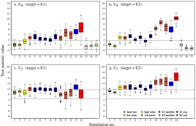
Fig. 3. Box plots forUR correlation (top panel) andUT distance (bottom panel) test statistics for each of the global land-only average
COSMOS simulation temperature series, compared to≈100 different pseudo-proxy temperature realizations (iteratively running through
the E1 and E2 ensemble members as targets – see text). The left panels are for E1 (“low” solar) as target, right E2 (“high” solar) as target. The 5 % two-sided significance levels are shown with dashed lines. Each box covers the 50 % interval between the lower and upper quartiles, with the median as a thick black line between. The simulations are: 1 = land-use changes, 2 = low solar, 3 = high solar, 4 = volcanoes, 5– 9 = E1, 10–12 = E2, 13 = average E1, 14 = average E2. The CTRL simulation (numbers 15–17) results are shown for theURanalysis but not
forUT, since they are then used as internal references. Note that the y-axis forUT is flipped to simplify any comparisons with theURbox
plots.
of the internal variability of the true climate, and the distance measureD2does not require white noise. However, the null hypothesis of the statistical tests is that forced simulations are equivalent to CTRL simulations, so for the described tests to have the prescribed type I error level, the unforced sim-ulations should be well represented by white noise. We in-vestigated the seriousness of this problem by calculating the lag-1 autocorrelation for the full 3000-yr CTRL simulation, both in terms of the proportion of global area with signifi-cant autocorrelations for various time resolutions, as well as the lag-1 autocorrelation for the global land-only series (see Supplement for further details). It was found that beyond a 20-yr time resolution,δi can be considered as white noise, in keeping with the statistical assumptions of Sect. 2 of Part 1. Hence, a non-overlapping 30-yr mean resolution, as used in the present analysis, should be able to keep the type I error of the tests under reasonable control in the model.
4 Model – (pseudo-proxy) data comparison
4.1 Global analysis
“true” climates or “truths” as possible, each ensemble mem-ber was used as the target in turn.
For each type of “truth”, ≈100 noise realizations were generated to produce yi and zi with a rotation in the five E1 target simulations (20 noise realizations for each simu-lation, 5×20 = 100) (Fig. 3a and c) and in the three E2 tar-get simulations (33 noise realizations for each simulation, 3×33 = 99) (Fig. 3b and d). Iteratively treating the E1 or E2 ensemble members as targets could cause the distributions to be hierarchical, in that the error distribution associated with different noise realizations could potentially be small in comparison with the difference between ensemble mem-bers (internal climate variability in the model). Hence, an identical analysis to this was conducted but with zero proxy noise added to the target temperatures, which revealed the E1 and E2 ensemble simulations to give results with little qual-itative spread (not shown). This satisfied the authors suffi-ciently that the spread of the distributions in Fig. 3 predom-inantly represents the uncertainty due to the pseudo-proxy noise realizations.
To further explain theUT andUR box plot distributions shown in Fig. 3, the first four represent the single forc-ing simulations, namely land-use changes (green), low so-lar (light orange), high soso-lar (yellow) and volcanoes (red), where they are compared with either the E1 (left panels) or the E2 (right panels) simulations as target. Analogously, the next five box plots (numbers 5–9) represent the E1 simula-tions, all coloured dark blue with their corresponding ensem-ble averageUR/UT value in blue (number 13). The three E2 simulations are coloured dark red (numbers 10–12) with their corresponding ensemble average in red (number 14). Note that, when an E1 (or E2) simulation is used as the target, this target simulation is excluded from the E1 (or E2) ensemble being analysed. Additionally, for comparison, Fig. 3a and b feature an analysis of the three CTRL simulation segments (numbers 15–17) as these are not required in the calculation ofUR.
From Fig. 3a and b, theURcorrelation analysis, it is clear that individual E1 and E2 ensemble members are signifi-cantly correlated with both E1 and E2 targets. However, the E2 simulations are the most highly correlated, whichever is the target. This can be expected in so far as the E2 simula-tions feature the strongest solar forcing and the largest vari-ability (Fig. 1). However, the significant correlations between E1 and E2 ensembles may not be reflected in a distance-based measure.UT is expected to be more effective in distin-guishing between the simulations and, in some instances, be-ing capable of rankbe-ing them. The principal reason bebe-ing that the correlation analysis does not consider the variance of two compared series (target and simulation), whereas this is ex-plicitly considered in the distance measure. This can be seen by the fact that, when E1 serves as target (Fig. 3c), E1 sim-ulations are generally significantly closer to the target than CTRL simulations, whilst the E2 simulations are not. The E1 and E2 simulations are also correctly distinguished when
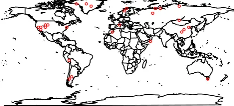
Fig. 4. The 27 proxy locations taken from Juckes et al. (2007) for the
present local-scale comparison. Note that the Juckes et al. (2007) set consists of 33 proxy locations, but some locations were so close together that a single representation was chosen for that location. A higher resolution model would likely have allowed a comparison using the full set of locations.
E2 serves as target. In this case, however, both are closer to the target than CTRL simulations (Fig. 3d).
The low solar single-forced simulation (number 2) is not significantly correlated with, or close to, the E1 targets (Fig. 3a and c). In contrast, the high solar simulation (num-ber 3) is significantly correlated with, and close to, the E2 targets (Fig. 3b and d). This implies that the low solar forc-ing is too weak to produce any detectable effect at the 30-yr time unit, whilst the high solar is strong enough. A related conclusion was reached by Ammann et al. (2007): the greater the solar forcing amplitude applied to their model, the weaker the detectable response to other natural forcings. In regard to CTRL simulations, theirUR values are mostly insignificant, as should be expected given the construction of the experi-ment and the null hypothesis being tested.
4.2 Local analysis
At global or hemispheric scales, the temperature can be ex-pected to respond to large-scale external forcings (such as so-lar or greenhouse gases), whereas at local or regional scales the internal climate dynamics can account for a larger pro-portion of the temperature variability (Goosse et al., 2005). Hence, on small spatial scales, the ability to distinguish be-tween simulations that use low and high solar forcing, and consequently rank them, may not be possible. A current set of proxy locations from Juckes et al. (2007) was used to gen-erate pseudo-proxies in order to investigate whether the low and high solar simulations can still be distinguished (Fig. 4). Though this set of locations is clearly a sparse representation of the global surface, 20–40 or so proxy locations is a typ-ical number of high quality millennial proxy data found in current analyses (Christiansen and Ljungqvist, 2011).
a. UR (target = E1)
ï2 0 2 4 6 8 10 12 14 16
1 2 3 4 5 6 7 8 9 10 11 12 13 14 15 16 17
b. UR (target = E2)
ï2 0 2 4 6 8 10 12 14 16
1 2 3 4 5 6 7 8 9 10 11 12 13 14 15 16 17
c. UT (target = E1)
8 6 4 2 0 ï2 ï4 ï6 ï8 ï10
1 2 3 4 5 6 7 8 9 10 11 12 13 14
d. UT (target = E2)
8 6 4 2 0 ï2 ï4 ï6 ï8 ï10
1 2 3 4 5 6 7 8 9 10 11 12 13 14
landïuse
low solar
high solar volcanoes
E1 member E2 member
E1 avg. E2 avg.
landïuse
low solar
high solar volcanoes
E1 member E2 member
E1 avg. E2 avg.
Simulation no.
T
est statistic v
alue
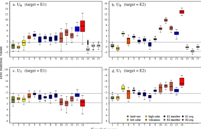
Fig. 5. As Fig. 3, but using the local proxy locations from Juckes et al. (2007).
before they are combined to obtain a single UR and UT value for each simulation (Sects. 7 and 8; Part 1). The cor-relation analysisURfor the Juckes et al. (2007) proxy loca-tions (Fig. 5a and b) gives similar results to the global time-series analysis, though surprisingly the correlations are not less significant, rather sometimes even more significant. This is something that could not have been expected due to the in-creased influence of internal (unforced) variability at the re-gional scale in combination with the reduced area coverage. However, in contrast to the global analysis, when E1 serves as target,UT is unable to distinguish the E1 simulations from the CTRL simulations (Fig. 5c), whereas the E2 simulations are again significantly closer to the target than the CTRL sim-ulations when E2 serves as target (Fig. 5d). Concerning the single forcing simulations, only the high solar (number 3) is significantly closer to the targets than the CTRL simulations when E2 is the target (Fig. 5d).
Using a realistic set of proxy locations such as the Juckes et al. (2007) set, it seems difficult to rank simulations, un-less the forcing is large and multi-decadal in nature (as is the case for the high solar forcing used here). Note thatUR is more sensitive thanUT for testing if a model forcing has any correspondence with the true climate, but it answers a dif-ferent question thanUT. This higher sensitivity is seen when we compare subfigures a and b with c and d respectively in both Figs. 3 or 5. Specifically, ifUR is not significant, nor is
UT. Comparisons between the Juckes et al. (2007) and global land-only average results naturally lead to the question of
how the possibility to rank simulations depends on the spatial coverage of the pseudo-proxy data.
5 Varying coverage
There are in practice relatively few locations which have high quality proxy data available or where there is the potential at present to acquire more data. A pseudo-proxy experiment, however, has the advantage of allowing any number of lo-cations to be used to serve as a proxy series or instrumen-tal series. Hence, an analysis is conducted on how varying degrees of % surface area coverage affect the sensitivity of the correlation and distance measures to distinguish between simulations with low or high solar forcing.
a. UR(target = E1)
ï
2
0
2
4
6
8
10
12
14
16
18
20
0.1 0.25 0.5 1 2 3 4 5
a. UR(target = E2)
ï
2
0
2
4
6
8
10
12
14
16
18
20
0.1 0.25 0.5 1 2 3 4 5
c. UT(target = E1)
420
ï
2
ï
4
ï
6
ï
8
ï
10
0.1 0.25 0.5 1 2 3 4 5
d. UT(target = E2)
420
ï
2
ï
4
ï
6
ï
8
ï
10
0.1 0.25 0.5 1 2 3 4 5
Percent of global surface area
T
est statistic v
alue
low solar high solar volcanoes
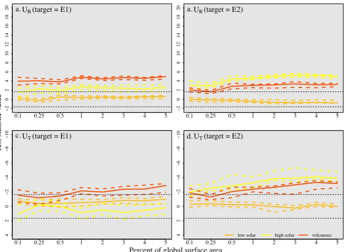
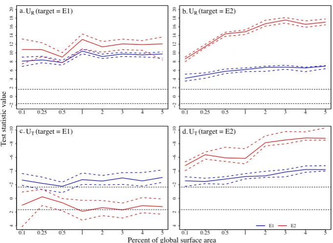
Fig. 6.URcorrelation (top panels) andUT distance (bottom panels) measures for volcanic (red), low (light orange) and high (yellow) solar
forcing simulations, against increasing % global surface area coverage. The left panels are for E1 as target, right panels E2 as target. The 5 % significance level is shown with dashed lines. The filled coloured lines denote the median value, with the dashed coloured lines representing the upper and lower quartiles.
was selected as a stratified random sample from the avail-able land points in the COSMOS simulations, with specified proportions for three strata (the latitudinal bands 0–30◦, 30–
60◦, 60–90◦). The stratification was chosen to better control the coverage and to account for the changing area of the grid points with latitude in the simulations.
Figure 6 shows the correlationUR(top panel) and distance
UT (bottom panel) measures for the low (light orange) and high solar (yellow) single forcing simulations for different % coverages, again with both E1 and E2 simulations serv-ing as targets. For each % coverage level, approximately 100 noise realizations were generated, of which the median val-ues are represented by solid lines and the upper and lower quartiles are dashed. For comparison, results for the volcanic (red) forcing simulation are also shown. The target and test statistics panels are arranged the same as Figs. 3 and 5.
The high solar simulation is significantly correlated even for the lowest coverages when E2 serves as target (Fig. 6b), whilst also achieving significantURvalues for coverages up-wards of 1 % when E1 serves as target. Contrastingly, the high solar simulationUT values are significantly better than the CTRL simulations for all coverages when E2 serves as target (Fig. 6d), but not for any coverage when E1 serves as target (Fig. 6c). The low solar simulation shows no signif-icant correlations for either target ensemble and can there-fore be expected to be indistinguishable from the CTRL sim-ulations using theUT measure. The volcanic simulation is
mostly significantly correlated with both E1 and E2 targets (Fig. 6a and b), but itsUT values are generally only signif-icant for coverages upwards of 1 % for both targets (Fig. 6c and d).
Figure 7 is arranged as Fig. 6 but shows the E1 (blue) and E2 (red) ensemble average results. Both ensembles are sig-nificantly correlated with all targets, even for the lowest data coverages. The results forUT are much the same as for the global analysis in Sect. 4.1, where the E1 and E2 ensem-bles can be correctly ranked with their respective targets. For coverages lower than 1 %, it becomes difficult to distinguish E1 from the CTRL simulations or separate the E1 and E2 simulations when E1 serves as target (Fig. 7c). Additionally, the experiments of Figs. 6 and 7 were conducted for cases with a SNR = 0.25 and also with negligible noise, the results of which are briefly discussed in the conclusions and shown in the Supplement. An important feature of note in Figs. 6 and 7 is how flat theUR andUT measures are with chang-ing % coverage after a certain coverage is reached. In fact, there is little gain in increasing the sample size from 40 or so proxy series to several hundred. Above all else, this suggests a substantial degree of spatial correlation in simulated tem-peratures, given the 30-yr time resolution used in this analy-sis (Jones et al., 1997; Franke et al., 2011).
a. UR(target = E1)
ï
2
0
2
4
6
8
10
12
14
16
18
20
0.1 0.25 0.5 1 2 3 4 5
b. UR(target = E2)
ï
2
0
2
4
6
8
10
12
14
16
18
20
0.1 0.25 0.5 1 2 3 4 5
c. UT(target = E1)
420
ï
2
ï
4
ï
6
ï
8
ï
10
0.1 0.25 0.5 1 2 3 4 5
d. UT(target = E2)
420
ï
2
ï
4
ï
6
ï
8
ï
10
0.1 0.25 0.5 1 2 3 4 5
Percent of global surface area
T
est statistic v
alue
E1 E2
Fig. 7. As Fig. 6, but for the E1 (blue) and E2 (red) ensemble averages.
different individual simulations before calculating theT and
UT statistics. This variant has been used in all analyses here. In the alternative variant, defined in Appendix A of Part 1, the averaging is instead undertaken on the simulation tem-perature series before calculating theD2. Results for vary-ing coverage with this alternative approach are shown in Ap-pendix A of this paper, where the Fig. A1 should be com-pared with Fig. 7c and d.
6 Conclusions
We apply a new statistical framework (Sundberg et al., 2012) designed for comparing ensemble model simulation sur-face temperature from one or more locations with proxy and instrumental data. This framework derives a unified correlation-based statistic (UR) that provides an initial test of whether a set of simulation time series from different lo-cations (and/or seasons) correlates with a set of target se-ries for the corresponding real locations (seasons), and a distance-based measure (UT) that can be used to assess the goodness-of-fit of a given forced simulation in compari-son with those that are unforced. The ultimate goal was to rank the simulations according to their closeness to the tar-get data. A pseudo-proxy experiment was designed for this task, based on the MPI-COSMOS Earth system model sim-ulations (Jungclaus et al., 2010). Here, the “true” climate and the proxy noise are known; hence, if no difference be-tween two forced simulations containing different solar forc-ing evolutions can be detected with these methods for realis-tic proxy noise levels, then no significant conclusions could
be assumed based on comparing the same model output with real proxy data.
Firstly, an analysis was conducted on globally averaged land-only data where a single series was calculated for each simulation and compared with every member of the full-forced E1 (with low solar) and E2 (with high solar) ensem-bles in turn plus added noise. Regardless of whether E1 or E2 simulations are used as a target, it was found that both simulation types are strongly correlated (significant positive
UR) with each other. Knowing that the shared forcing infor-mation gives significantly correlated temperature evolutions between both low and high solar simulations,UT was found capable of ranking these simulations correctly.
a. UT(target = E1)
420
ï
2
ï
4
ï
6
ï
8
ï
10
ï
12
ï
14
ï
16
0.1 0.25 0.5 1 2 3 4 5
b. UT(target = E2)
420
ï
2
ï
4
ï
6
ï
8
ï
10
ï
12
ï
14
ï
16
0.1 0.25 0.5 1 2 3 4 5
Percent of global surface area
T
est statistic v
alue
E1 E2 E1 inside E2 inside
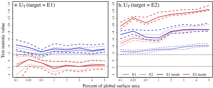
Fig. A1. As Fig. 7, with E1 (blue) and E2 (red) ensemble averages. The thick lines denote the use of inside averaging, whilst the thin lines
denote outside averaging (as presented in Fig. 7). Note that the y-axis is extended here to accommodate the inside averaging lines.
series are needed. Additionally, the same type of analysis was conducted for a higher noise level (SNR = 0.25), where it was found that the E1 and E2 simulations are indistinguish-able even if the global surface area coverage is 5 % (approxi-mately 230 proxy locations). Although these results, in quan-titative terms, are conditional upon the actual climate model simulations used to define the pseudo-proxy world, they have an important implication: it is more important to improve the quality of individual local proxy series in terms of SNR than it is to increase the quantity of available proxy locations. Even a limited spatial coverage is sufficient to distinguish forced multi-decadal temperature signals, provided the tem-perature proxies are of a sufficient quality and represent areas that can be directly compared with model output.
Appendix A
Averaging insideD2
From Fig. A1, if the alternative “inside” averaging (defined in Appendix A of Part 1; thick lines) is used instead of “out-side” averaging (thin lines) in calculating the E1 and E2 en-semble averages, theUT results appear to change little if E1 serves as target, whereas there is a substantial increase in the significance ofUT when E2 serves as target. This likely reflects the fact that, if there is a stronger common signal amongst the ensemble members (as with the high solar E2 ensemble), then the inside averaging approach will enhance the SNR of the series, whilst, if the common signal is weaker (as with the low solar E1 ensemble), there will not be a large difference between the approaches. Hence, inside averaging can be more effective than outside averaging.
Supplementary material related to this article is available online at: http://www.clim-past.net/8/1355/ 2012/cp-8-1355-2012-supplement.pdf.
Acknowledgements. This research was funded by the Swedish
Research Council (grants 70454201, 90751501 and B0334901) and the European Union (FP6 grant 017008, “Millennium” project). We thank Johann Jungclaus of the Max Planck Institute for providing the COSMOS data as well as help and advice regarding the simulations. We also thank G. Hegerl, Y. H. Yamazaki and an anonymous reviewer for constructive comments and advice in their reviews of the discussion paper.
Edited by: P. Brohan
References
Ammann, C. M., Joos, F., Schimel, D. S., Otto-Bliesner, B. L., and Tomas, R. A.: Solar influence on climate during the past millen-nium: Results from transient simulations with the NCAR Climate System Model, P. Natl. Acad. Sci., 104, 3713–3718, 2007. Bard, E., Raisbeck, G., Yiou, F., and Jouzel, J.: Solar irradiance
dur-ing the last 1200 years based on cosmogenic nuclides, Tellus B, 52, 985–992, 2000.
Brohan, P., Kennedy, J. J., Harris, I., Tett, S. F. B., and Jones, P. D.: Uncertainty estimates in regional and global observed tempera-ture changes: A new data set from 1850, J. Geophys. Res., 111, D12106, doi:10.1029/2005JD006548, 1–12, 2006.
Christiansen, B. and Ljungqvist, F. C.: Reconstruction of the extra-tropical NH mean temperature over the last millennium with a method that preserves low-frequency variability, J. Climate, 24, 6013–6034, 2011.
Christiansen, B. and Ljungqvist, F. C.: The extra-tropical North-ern Hemisphere temperature in the last two millennia: recon-structions of low-frequency variability, Clim. Past, 8, 765–786, doi:10.5194/cp-8-765-2012, 2012.
Cliver, E. W., Boriakoff, V., and Feynman, J.: Solar variability and climate change: a geomagnetic and aa index and global surface temperature, Geophys. Res. Lett., 25, 1035–1038, 1998. Feulner, G.: Are the most recent estimates for Maunder Minimum
Folland, C. K., Rayner, N. A., Brown, S. J., Smith, T. M., Shen, S. S. P., Parker, D. E., Macadam, I., Jones, P. D., Jones, R. N., Nicholls, N., and Sexton, D. M. H.: Global temperature change and its uncertainties since 1861, Geophys. Res. Lett., 28, 2621– 2624, 2001.
Franke, J., Gonzalez-Rouco, J. F., Frank, D., and Graham, N. E.: 200 years of European temperature variability: insights from and tests of the proxy surrogate reconstruction analog method, Clim. Dynam., 37, 133–150, 2011.
Goosse, H., Renssen, H., and Bradley, R. S.: Internal and forced cli-mate variability during the last millennium: a model-data com-parison using ensemble simulations, Quaternary Sci. Rev., 24, 1345–1360, 2005.
Gray, L. J., Beer, J., Geller, M., Haigh, J. D., Lockwood, M., Matthes, K., Cubasch, U., Fleitmann, D., Harrison, G., Hood, L., Luterbacher, J., Meehl, G. A., Shindell, D., van Geel, B., and White, W.: Solar influences on climate, Rev. Geophys., 48, RG4001, doi:10.1029/2009RG000282, 2010.
Hoyt, D. V. and Schatten, K. H.: A discussion of plausible solar irradiance variations, J. Geophys. Res., 98, 18895–18906, 1993. Jones, P. D., Osborn, T. J., and Briffa, K. R.: Estimating Sampling Errors in Large-Scale Temperature Averages, P. Natl. Acad. Sci., 10, 2548–2568, 1997.
Jones, P. D., Briffa, K. R., Osborn, T. J., Lough, J. M., van Om-men, T. D., Vinther, B. M., Luterbacher, J. W. E. R. Z. F. W., Mann, M. E., Schmidt, G. A., Ammann, C. M., Buckley, B. M., Cobb, K. M., Esper, J., Goosse, H., Graham, N., Janse, E., Kiefer, T., Kull, C., K¨uttel, M., Mosley-Thompson, E., Overpeck, J. T., Riedwyl, N., Schulz, M., Tudhope, A. W., Villalba, R., Wanner, H., Wolff, E., and Xoplaki, E.: High-resolution palaeoclimatol-ogy of the last millennium: a review of current status and future prospects, Holocene, 19, 3–49, 2009.
Juckes, M. N., Allen, M. R., Briffa, K. R., Esper, J., Hegerl, G. C., Moberg, A., Osborn, T. J., and Weber, S. L.: Millennial temper-ature reconstruction intercomparison and evaluation, Clim. Past, 3, 591–609, doi:10.5194/cp-3-591-2007, 2007.
Jungclaus, J. H., Lorenz, S. J., Timmreck, C., Reick, C. H., Brovkin, V., Six, K., Segschneider, J., Giorgetta, M. A., Crowley, T. J., Pongratz, J., Krivova, N. A., Vieira, L. E., Solanki, S. K., Klocke, D., Botzet, M., Esch, M., Gayler, V., Haak, H., Raddatz, T. J., Roeckner, E., Schnur, R., Widmann, H., Claussen, M., Stevens, B., and Marotzke, J.: Climate and carbon-cycle variability over the last millennium, Clim. Past, 6, 723–737, doi:10.5194/cp-6-723-2010, 2010.
Knutti, R. and Hegerl, G. C.: The equilibrium sensitivity of the Earth’s temperature to radiation changes, Nat. Geosci., 1, 735– 743, 2008.
Krivova, N. A., Balmaceda, L., and Solanki, S. K.: Reconstruction of solar total irradiance since 1700 from the surface magnetic flux, Astron. Astrophys., 467, 335–346, 2007.
Lean, J., Beer, J., and Bradley, R.: Reconstruction of solar irradiance since 1610: Implications for climate change, Geophys. Res. Lett., 22, 3195–3198, 1995.
Lockwood, M.: Shining a light on solar impacts, Nat. Clim. Change, 1, 98–99, 2011.
Marsland, S. J., Haak, H., Jungclaus, J. H., Latif, M., and Roeske, F.: THe Max Planck Institute global ocean/ice model with orthogo-nal curvilinear coordinates, Ocean Modell., 5, 91–127, 2003.
Reid, G. C.: Solar total irradiance variations and the global sea sur-face temperature record, J. Geophys. Res., 96, 2835–2844, 1991. Reid, G. C.: Solar forcing and the global climate change since the
mid-17th century, Climate Change, 37, 391-405, 1997.
Roeckner, E., B¨auml, G., Bonaventura, L., Brokopf, R., Esch, M. G., Hagemann, S., Kirchner, I., Kornblueh, L., Manzini, E., Rhodin, A., Schlese, U., Schulzweida, U., and Tompkins, A.: The atmospheric general circulation model ECHAM5, Part I: Model description, Technical Report, Max Planck Institute of Meteorol-ogy, 349, available from MPI for MeteorolMeteorol-ogy, Hamburg, Ger-many, 127 pp., 2003.
Schmidt, G. A., Jungclaus, J. H., Ammann, C. M., Bard, E., Bra-connot, P., Crowley, T. J., Delaygue, G., Joos, F., Krivova, N. A., Muscheler, R., Otto-Bliesner, B. L., Pongratz, J., Shindell, D. T., Solanki, S. K., Steinhilber, F., and Vieira, L. E. A.: Climate forc-ing reconstructions for use in PMIP simulations of the last mil-lennium (v1.0), Geosci. Model Dev., 4, 33–45, doi:10.5194/gmd-4-33-2011, 2011.
Schrijver, C. J., Livingston, W. C., Woods, T. N., and Mewaldt, R. A.: The minimal solar activity in 2008–2009 and its impli-cations for long-term climate modeling, Geophys. Res. Lett., 38, L06701, doi:10.1029/2011GL046658, 2011.
Servonnat, J., Yiou, P., Khodri, M., Swingedouw, D., and Denvil, S.: Influence of solar variability, CO2and orbital forcing between 1000 and 1850 AD in the IPSLCM4 model, Clim. Past, 6, 445– 460, doi:10.5194/cp-6-445-2010, 2010.
Shapiro, A. I., Schmutz, W., Rozanov, E., Schoell, M., Haberreiter, M., Shapiro, A. V., and Nyeki, S.: A new approach to the long-term reconstruction of the solar irradiance leads to large histori-cal solar forcing, Astron. Astrophys., 529, 1–8, 2011.
Smerdon, J. E.: Climate models as a test bed for climate reconstruc-tion methods: pseudoproxy experiments, WIREs Clim. Change, 3, 63–77, doi:10.1002/wcc.149, 2012.
Steinhilber, F., Beer, J., and Fr¨ohlich, C.: Total solar irradi-ance during the Holocene, Geophys. Res. Lett., 36, L19704, doi:10.1029/2009GL040142, 2009.
Sundberg, R., Moberg, A., and Hind, A.: Statistical framework for evaluation of climate model simulations by use of climate proxy data from the last millennium – Part 1: Theory, Clim. Past, 8, 1339–1353, doi:10.5194/cp-8-1339-2012, 2012.
Tapping, K. F., Boteler, D., Charbonneau, P., Crouch, A., Manson, A., and Paquette, H.: Solar magnetic activity and total irradiance since the Maunder Minimum, Solar Phys., 246, 309–326, 2009. Wang, Y.-M., Lean, J. L., and Sheeley, N. R.: Modeling the Sun’s
magnetic field and irradiance since 1713, Astrophys. J., 625, 522–538, 2005.
Yoshimori, M., Stocker, T. F., Raible, C. C., and Renold, M: Ex-ternally forced and internal variability in ensemble climate sim-ulations of the Maunder Minimum, J. Climate, 18, 4253–4270, 2005.