Brief communication “On one mechanism of low frequency variability of the Antarctic Circumpolar Current”

(1)

Nonlin. Processes Geophys., 18, 361–365, 2011 www.nonlin-processes-geophys.net/18/361/2011/ doi:10.5194/npg-18-361-2011

Nonlinear Processes

in Geophysics

Brief communication

“On one mechanism of low frequency variability of the Antarctic

Circumpolar Current”

O. G. Derzho1,2and B. de Young1

1_{Department of Physics and Physical Oceanography, Memorial University of Newfoundland, St. John’s, NL,} A1B 3X7, Canada

2_{Institute of Thermophysics, Russian Academy of Sciences, 630090 Novosibirsk, Russia}

Received: 14 February 2011 – Revised: 26 May 2011 – Accepted: 2 June 2011 – Published: 16 June 2011

Abstract. In this paper we present a simple analytical model for low frequency and large scale variability of the Antarc-tic Circumpolar Current (ACC). The physical mechanism of the variability is related to temporal and spatial variations of the cyclonic mean flow (ACC) due to circularly propagating nonlinear barotropic Rossby wave trains. It is shown that the Rossby wave train is a fundamental mode, trapped be-tween the major fronts in the ACC. The Rossby waves are predicted to rotate with a particular angular velocity that de-pends on the magnitude and width of the mean current. The spatial structure of the rotating pattern, including its zonal wave number, is defined by the specific form of the stream function-vorticity relation. The similarity between the sim-ulated patterns and the Antarctic Circumpolar Wave (ACW) is highlighted. The model can predict the observed sequence of warm and cold patches in the ACW as well as its zonal number.

1 Introduction

The Antarctic Circumpolar current (ACC) is a strong flow transporting about 130 Sverdrups. It encircles the Antarctica thus connecting waters between the Atlantic, Pacific, and In-dian Oceans. Available observations suggest that the ACC contains a series of sharp temperature and density fronts, each separating two distinct water masses. Two major cir-cular fronts in the ACC are the Subantarctic Front (SAF) and the Polar Front (PF), whose mean paths are now well de-fined (Gille, 1994). The ACC flow varies with time and its variability can be divided into the short-timescale variabil-ity due to the local effect of mesoscale eddies (e.g. Sarukha-nian, 1985) and lower-frequency variability at greater

spa-Correspondence to: O. G. Derzho ([email protected])

tial extent. In this paper, we will focus on effects related to lower-frequency variability, which has the potential to in-fluence larger-scale ocean flow and climate variability. An example of such low-frequency variability is the Antarctic Circumpolar Wave (ACW) discovered by White and Peter-son (1996) and Jacobs and Mitchell (1996). The ACW con-sists of anomalies in sea-surface temperature, sea-level pres-sure, and sea-ice extent (Connolley, 2003) that propagate eastward around the Southern Ocean because of advection by the ACC.

(2)

362 O. G. Derzho and B. de Young: Low frequency variability of the ACC issues. Our aim is to show that the Rossby wave train

be-tween the SAF and PF is a fundamental mode of motion in the Southern ocean, and to present a simple mathematical model for this mode. Indeed, only the fundamental mode of motion can be sustained for long periods of time under vary-ing ambient conditions and complicated atmosphere-ocean interactions. A model for this fundamental mode, including prediction that zonal number for the patterns is likely to be 2 or 3, with intermittent warm and cold patches, is the major result of the paper.

2 Simplified theory

We consider the two-dimensional flow of a purely barotropic fluid, which is rotated with an angular velocitycaround a ge-ographical pole in a circular channel of the widthL. We use the gamma plane approximation, which means that the exact expression for the Coriolis force is expanded about a pole. This approach differs from the widely used beta plane ap-proximation where expansions are about some mid-latitude location. We introduce the stream function in the usual way u=ψξ,vξ= −ψφ, whereu,vare velocities in the eastward

and the northward directions;ξ is dimensionless radial dis-tance to the geographical pole scaled with the channel width

L; φ is the longitude. Our idea is that a circular channel created by the SAF and PF acts like a waveguide with non-penetratable boundaries. The dimensionless equation for the stream functionψ in this case is the following e.g. Derzho and Afanasyev (2008),

∇2ψ− ε

2

Ro ξ2

2 =F (ψ−c

ξ2

2), ε=L/RE1, (1) whereF is an arbitrary function to be determined from the relation between the potential vorticity and the stream func-tion at some cross secfunc-tions of the flow. As it follows from the latter inequality, we consider the length scale of the flow to be much smaller that the radius of the EarthRE.Ro=U/2Lis the Rossby number,denotes the rotation rate of the Earth,

U is a typical circumferential velocity. We also use the hy-drostatic and rigid lid approximations. The validity of these approximations for the problem was discussed by Derzho and de Young (2011). Classical papers like Stern (1975) as-sumed that F is linear. We will assume that the potential vorticity-stream function relationF has a weakly nonlinear functional form thus extending the classical approach.

F= −λ(ψ−cξ

2

2 )+σ

2_{f (ψ}₋_cξ2

2 ), σ1, (2)

whereλis a constant andfdetermines the functional nonlin-earity in the vorticity-stream function relation. That weakly nonlinear relation was experimentally confirmed by Derzho and Afanasyev (2008). Here we focus on the solutions of Eq. (1) whose radial variations appear at much shorter scales

compared to the angular oneψ=ψ (ξ,8), 8=σ φ. We seek asymptotic solutions of Eqs. (1, 2) in the form of power series in the small parameterσ2. We look for solutions of Eqs. (1, 2) in a circular channel with inner and outer rigid boundaries located atξ=R1 andξ=R2, respectively. As shown by Derzho and de Young (2011), the regular zeroth order solu-tion of Eqs. (1, 2) satisfying the boundary condisolu-tions has the form,

ψ(0)=(ξ

2

2 − 2

λ)( ε2

λ Ro +c)+A(8) W (ξ ), (3)

where the functionAin Eq. (3) is to be determined from the solvability condition to the first approximation. The constant

λand functionW (ξ )can be determined for given valuesR1 andR2as shown in Derzho and de Young (2011). The first term in Eq. (3) has physical meaning of an ambient mean cur-rent, which is the ACC in our study. The second term denotes a disturbance superimposed on that current, it corresponds to the ACW-like pattern in our application. It can be shown from Eq. (3) that the mean current is approximated as the cur-rent with a constant angular velocity. The non-dimensional expression for that velocitycmand its dimensional

counter-part,cm,dim, are the following,

c_m= ε

2

Ro λ+c, cm,dim= L2

R_E2

2

λ +cdim. (4)

(3)

O. G. Derzho and B. de Young: Low frequency variability of the ACC 363

Derzho and de Young: Low frequency variability of the ACC

5

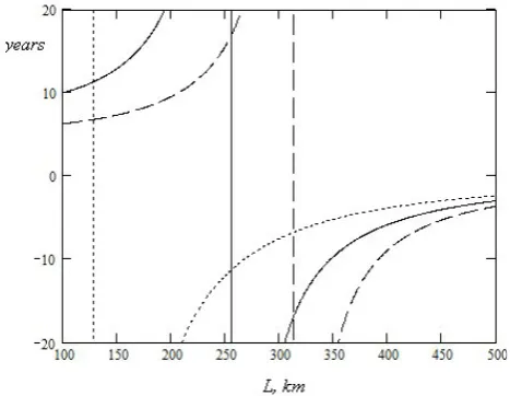
Fig. 1. Period of rotation of the Rossby wave train in years versus the waveguide width (mean distance between the SAF and PF), in km for different magnitudes of the mean current: 2 cm/s - dots, 8 cm/s - solid line, 12 cm/s - dash line. The negative period indicates that the Rossby wave train propagates against the mean current

Fig. 2.Maximum dimensional circumferential velocity at the outer circumference (3760 km) versuss1for mode numbersN= 1,2,3

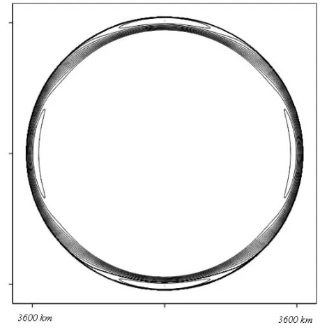
Fig. 3. The streamline pattern for the quadrupole case (N= 2);

s1= 0.912

Fig. 1. Period of rotation of the Rossby wave train in years versus

the waveguide width (mean distance between the SAF and PF), in km for different magnitudes of the mean current: 2 cm s−1– dots, 8 cm s−1– solid line, 12 cm s−1– dash line. The negative period indicates that the Rossby wave train propagates against the mean current

f (B)=s1B+s2B2,A88 =I0+A I1+A2I2, (5) whereI0,I1, andI2are constants that depend ons1,s2,c, and

cm.

Numerical analysis of Eq. (5) along with the condition of zero circulation leads to the expression for the Rossby wave amplitude as function of longitude. Analytical results for the case with zero mean flow were presented in Derzho and de Young (2011), these results are extended here for the more realistic case with ambient mean current. Equation (5) has solutions in the form of cnoidal waves with the wavelength

2π

N (for the original angular coordinateφ,N=1,2,...where

Nis the zonal number. Our specific choice ofNcorresponds to a 2N-pole. Similarly to Derzho and de Young (2011), it can be shown that the problem has a unique solution onces1,

s2, and the magnitude of the ambient shear are prescribed. That is the wave amplitude and spatial structure are com-pletely and uniquely defined by the specific form of the vorticity-stream function relation and the magnitude and the width of the ambient current.

3 Application to the ACC conditions

Here we present our calculations for the special case of a vor-tical pattern rotating around the Antarctic aimed at explain-ing a mechanism for slow frequency and large scale variabil-ity of the ACC. Our solution for a vortical pattern in a polar region consists of two parts, the first part is a Rossby wave while the second part is a current. Our physical assumption is that the Subantarctic Front (SAF) and the Polar Front (PF),

which are reasonably well-defined narrow jets (about 40 km wide) create a wave guide for a Rossby wave train. Gille (1994) analyzed GEOSAT altimetry data and presented the mean paths of the SAF and PF jets. Although topography affects the tracks of these paths, they remain quite close to-gether around the Antarctic continent. According to Fig. 9 from Gille (1994) the distance between mean SAF and PF paths varies from about 100 km to more than 500 km in some parts of the South Indian Ocean. However, since these dis-tances are much smaller than the distance from either SAF and PF to the South pole, the SAF and PF paths can be ap-proximated as two circumferences. As the SAF and PF sep-arate distinct water masses, we conceptualize them as rigid boundaries, which create a circular channel. In our calcu-lations, we choose the internal circumference at which the radial velocity is zero to be located at 3400 km. First, it is interesting to note that according to Eq. (4) the angular ve-locity of rotation of the vortical structure is independent of the zonal number. This conclusion is supported by the fre-quency domain decomposition of the interannual variability in the Southern Ocean performed by Venegas (2003), where variability was detected with time scale of 5 yr for the zonal mode 2 and 3.3 yr, for the zonal mode 3, respectively. The re-sulting period of rotation for the whole patterns is then 10 yr, same for both zonal modes 2 and 3. As can be seen from Eq. (4), the period of rotation of the vortical pattern (Rossby wave train) is independent of the specific coefficientsσ,s1,

(4)

364 O. G. Derzho and B. de Young: Low frequency variability of the ACC

Derzho and de Young: Low frequency variability of the ACC

5

s1= 0.912

Fig. 2. Maximum dimensional circumferential velocity at the outer

circumference (3760 km) versuss1for mode numbersN=1,2,3

variability of the ACC reported in White and Peterson (1996) who suggested periods of 8–9 yr. As the wave guide is quite narrow, so there is no much difference between the mean cur-rent magnitudes at the inner and the outer boundaries of the waveguide according to Eq. (3). Our choice for the magni-tude of the ambient current and the length scale leads to a flow rate of 121 Sv if we assume that that the average depth of the oceans is 4 km. This value is close to 130 Sv, the flow rate in the ACC, reported by many authors. It can be shown (Derzho and de Young, 2011) that solutions to our problem can only exist ifs2<0. Here we examine the cases2= −1 and setσ=0.3; these parameters affect the magnitude of the velocity field in the wave for givens1. We will show below that this choice of parameters lead to reasonable agreement with observations. With all these parameters are set, it is straightforward to analytically determine possible values of

s1 for which stationary rotating vortex patterns exist. Ba-sically, in the present model, we aggregate many physical effects into a couple of coefficients in the vorticity-stream function relation. The advantage of such approach lies in simplicity as separate parameterisation of many complicated processes, in particular, the ocean-atmosphere interactions, leads to accumulation of inaccuracies associated with each parameterisation.

In Fig. 2, we present the maximum dimensional circumfer-ential velocity at the outer circumference versuss1for vari-ous zonal mode numbers N=1,2,3. The maximal radial velocities are not shown as they are much smaller than the circumferential ones. It can be seen that regions of existence for different zonal modes are separated. There are intervals where the only mode 1 or mode 2 only can exist. Regions of existence for modes 2 and 3 can overlap. But if mode 3 is excited, it is unlikely that the mode 2 exists at the same value ofs1as the mode 2 pattern should produce quite large flow velocities.

Again, we recall that the leading order stream function patterns can be found from Eqs. (3), (4), (5). These pat-terns are shown in Fig. 3 for the case of quadrupole (N=2);

Derzho and de Young: Low frequency variability of the ACC 5

s1= 0.912

Fig. 3. The streamline pattern for the quadrupole case (N=2); σ=0.3,s1=0.912

s1=0.912 . The pattern is quite symmetric and the actual cnoidal Rossby wave train is close to a sinusoidal packet. However, this does not mean that the linear theory can pre-dict properties of such flow, actually our theory prepre-dicts that there is a unique amplitude that satisfies our mathematical formulation for the prescribed set of parameters. Linear the-ories are unable to predict an amplitude of the wave and con-sequently do not predict the magnitude of the velocity field in it. For the mentioned set of parameters, we calculated that the maximum of the circumferential velocity due to the waves is 15 cm s−1, while the magnitude of the the radial velocity is 1 cm s−1. We also note that the variation ofσdoes not qual-itatively change the results. For example, whenσ=0.3 and

s1=0.912, the predicted Rossby wave pattern has exactly the same velocity field as forσ=0.1 ands1=8.208.

(5)

O. G. Derzho and B. de Young: Low frequency variability of the ACC 365 4 Conclusions

Here we modeled the variability of the ACC due to nonlin-ear Rossby wave trains with zero circulation. The train is predicted to rotate around the Antarctica. The angular ve-locity of rotation of the vortical Rossby wave pattern is not arbitrary, but is predicted to be at a specific rate, which is in-dependent of the zonal number but rather depends on the dis-tance between the SAF and PF, and the strength of the mean current. The pattern propagates against the ACC for large distances between the SAF and PF and collateral to the ACC when this distance is short. Once the vorticity-stream func-tion relafunc-tion is prescribed, our model predicts that there is a unique nonlinear vortex pattern for each zonal mode num-ber. Various modes are allowed to exist, however they have reasonable amplitudes (those leading to the observed veloci-ties) in different range of parameters in the stream function-vorticity relation, perhaps indicating that they are driven by different physical mechanisms. This conclusion is consistent with observations reported by Venegas (2003). Reasonable values for the distance between the SAF and PF and the mag-nitude of the average mean current lead to reasonable agree-ment for the period of rotation and the velocity field charac-teristics. The theory also predicts that the Rossby wave pat-terns include patches of trapped fluid that could carry fluid from the inner (colder) and outer (warmer) boundaries of the ACC thus explaining the sequence of the warm and cool patches carried by the ACW. A more detailed modeling of the ACC and ACW would require a spatially explicit numerical model, which is beyond the scope of the present study. We also believe that the detailed account of the spatial features, e.g. bathymetry, would not qualitatively change the main idea of the proposed mechanism for the low frequency variability of the ACC.

Acknowledgements. Constructive suggestions by the reviewers are

gratefully acknowledged.

Edited by: J. M. Redondo

Reviewed by: W.-G. Fruh and P. Fraunie

References

Cai, W., Baines, P. G., and Gordon, H. B.: Southern mid- to high-latitude variability, a zonal wavenumber-3 pattern, and the Antarctic Circumpolar Wave in the CSIRO coupled model, J. Cli-mate, 12, 3087–3104, 1999.

Connolley, W. M.: Long term variation of the antarctic circumpolar wave, J. Geophys. Res., 108 (C4), 8076–8098, 2003.

Derzho, O. G. and Afanasyev, Y. D.: Rotating dipolar gyres on a gamma-plane, Phys. Fluids, 20, 036603, 2008.

Derzho, O.G. and de Young, B.: Rotating nonlinear vortical patterns on a gamma plane, Stud. Appl. Math.,126, 186–201, 2011. Gille, S. T.: Mean sea surface height of the antarctic circumpolar

current from geosat data: methods and application, J. Geophys. Res., 99(C9), 18255–18273, 1994.

Jacobs, G. A. and Mitchell, J. L.: Ocean circulation variations asso-ciated with the antarctic circumpolar wave, Geophys. Res. Lett., 23, 2947–2950, 1996.

Rintoul, S. R., Hughes, C. W., and Olbers, D.: The Antarctic Cir-cumpolar Current system, in: Ocean Circulation and Climate, edited by: Siedler, G., Church, J., and Gould, J., International Geophysical Series, Academy Press, New York, 271–302, 2001. Sarukhanian, E. I.: Structure and Variability of the Antarctic

Cir-cumpolar Current, Oxonian Press, New Delhi, 1985.

Stern, M.: Minimal properties of planetary eddies, J. Mar. Res., 33, 1–13, 1975.

Venegas, S. A.: The Antarctic Circumpolar Wave: A Combination of Two Signals?, J. Climate, 16, 2509–2525, 2003.