www.ocean-sci.net/9/867/2013/ doi:10.5194/os-9-867-2013
© Author(s) 2013. CC Attribution 3.0 License.
Ocean Science
Optimal adjustment of the atmospheric forcing parameters of ocean
models using sea surface temperature data assimilation
M. Meinvielle, J.-M. Brankart, P. Brasseur, B. Barnier, R. Dussin, and J. Verron
Laboratoire des Ecoulements Géophysiques et Industriels, CNRS/Université de Grenoble, France
Correspondence to: M. Meinvielle ([email protected])
Received: 4 June 2012 – Published in Ocean Sci. Discuss.: 20 July 2012
Revised: 4 September 2013 – Accepted: 10 September 2013 – Published: 17 October 2013
Abstract. In ocean general circulation models, near-surface
atmospheric variables used to specify the atmospheric boundary condition remain one of the main sources of error. The objective of this research is to constrain the surface forc-ing function of an ocean model by sea surface temperature (SST) data assimilation. For that purpose, a set of corrections for ERAinterim (hereafter ERAi) reanalysis data is estimated for the period of 1989–2007, using a sequential assimilation method, with ensemble experiments to evaluate the impact of uncertain atmospheric forcing on the ocean state. The control vector of the assimilation method is extended to atmospheric variables to obtain monthly mean parameter corrections by assimilating monthly SST and sea surface salinity (SSS) cli-matological data in a low resolution global configuration of the NEMO model. In this context, the careful determination of the prior probability distribution of the parameters is an important matter. This paper demonstrates the importance of isolating the impact of forcing errors in the model to perform relevant ensemble experiments.
The results obtained for every month of the period between 1989 and 2007 show that the estimated parameters produce the same kind of impact on the SST as the analysis itself. The objective is then to evaluate the long-term time series of the forcing parameters focusing on trends and mean error cor-rections of air–sea fluxes. Our corcor-rections tend to equilibrate the net heat-flux balance at the global scale (highly positive in ERAi database), and to remove the potentially unrealis-tic negative trend (leading to ocean cooling) in the ERAi net heat flux over the whole time period. More specifically in the intertropical band, we reduce the warm bias of ERAi data by mostly modifying the latent heat flux by wind speed in-tensification. Consistently, when used to force the model, the corrected parameters lead to a better agreement between the mean SST produced by the model and mean SST observa-tions over the period of 1989–2007 in the intertropical band.
1 Introduction
Near-surface variables from atmospheric reanalyses (air tem-perature and humidity, wind speed, downward radiation and precipitation) are commonly used to specify surface bound-ary condition in ocean general circulation models (hereafter OGCMs) required for operational forecasts, ocean reanal-yses, or hindcast simulations of the recent ocean variabil-ity (the last 50 yr). However, these atmospheric variables are characterized by significant uncertainties at global scale as shown in different studies, such as Milliff et al. (1999), Wang and McPhaden (2001), Smith et al. (2001) or Sun et al. (2003). For example, the use of two different databases (e.g. from numerical weather prediction centers like ECMWF or NCEP) to compute the mean ocean–atmosphere net heat flux can lead to discrepancies on the order of at least 10 W m−2, while the signal of a global warming of the world ocean cor-responds to a value of 0.5 W m−2(Josey, 2011). It is there-fore important to reduce the atmospheric variables uncertain-ties in order to obtain better agreement between the models and the real ocean. Sea surface temperature (SST) is more accurately observed from space than most near-surface at-mospheric variables or air–sea fluxes assimilated in atmo-spheric models to construct the reanalyses. Although SST is used as boundary conditions in these atmospheric models, large errors remain in the produced surface atmospheric pa-rameters due to bulk formulae and radiative transfers model uncertainties. In OGCMs, observed values of SST (intrinsi-cally linked to air–sea exchanges) are not used in the surface forcing except when explicitly assimilated. In brief, models do not benefit, in their forcing, from one of the best observed ocean surface variables.
however to some inconsistency between the “assimilated” solution of the model and the “forced” one, and to the re-jection of the information contained in the SST. Since atmo-spheric forcing and particularly atmoatmo-spheric variables are an important source of surface errors, an alternative is to use SST data assimilation to constrain the surface atmospheric input variables of the atmospheric reanalyses. The aim is to correct the source of errors and not the consequence. An im-provement of fluxes estimation is crucial to perform realis-tic ocean simulations and can also help improving the atmo-spheric reanalyses since their atmoatmo-spheric state estimation could benefit from the link with the ocean dynamics via the ocean model. Moreover, this approach proposes an alterna-tive to other corrections of atmospheric forcing realized fol-lowing ad hoc considerations (e.g. Large and Yeager, 2004; Brodeau et al., 2010).
This idea has been explored in previous studies using two different types of data assimilation schemes. On the one hand, Stammer et al. (2004) used a four-dimensional varia-tional data assimilation scheme by including air–sea fluxes in the control vector. Over a ten-year period, they assimilated a large variety of oceanic observations, computed air–sea flux corrections, and carried out an important validation effort to compare the corrected fluxes to other independent estimates. This pioneering work was the first to demonstration that it is possible to make estimates of the atmospheric forcing fields by ocean data assimilation in a realistic case, even if the au-thors also show that the forcing correction may sometimes compensate for other errors in the ocean model. On the other hand, fluxes corrections can also be computed using sequen-tial assimilation methods. These methods are widely used in ocean data assimilation systems, and are easier to imple-ment than their variational counterpart. Skachko et al. (2009) and Skandrani et al. (2009) explored the capability of such methods to estimate forcing parameters corrections by us-ing ocean observations data. On the basis of a reduced or-der Kalman filter, they carried out idealized experiments that differ from the parameters included in the control vector, the construction of the synthetic observations to be assimilated, and the construction of initial condition. They showed that in an idealized case where errors are assumed to be entirely due to forcing parameters, it is possible to implement a se-quential data assimilation method to estimate objective cor-rections of these parameters. While Skachko et al. (2009) used temperature and salinity profiles that simulate the hor-izontal and temporal distribution of Argo floats in twin ex-periments, Skandrani et al. (2009) assimilated sea surface temperature and sea surface salinity extracted from a Mer-cator Ocean reanalysis (Ferry et al., 2010). The first study by Skachko et al. (2009) showed that this procedure leads to ac-curate estimations of parameters included in the control vec-tor, and following these first results, Skandrani et al. (2009), in a more realistic context, estimated forcing parameters cor-rections leading to reduced differences between the free sim-ulation and the reanalysis. However, these two studies also
suggest that the other sources of model errors (due to the coarse resolution or to the initial condition for example) can lead to unrealistic forcing parameters corrections and must be considered very carefully. In particular, they point out the importance of a proper determination of the prior probability distribution of forcing parameters and of their associated er-ror covariance matrix to obtain good parameters estimation. These results are thus an appropriate starting point for further developments of this approach, investigating its feasibility in a more realistic context. In this case the sources of errors are more diverse and require particular attention.
The purpose of this research is thus to constrain (within observation-based air–sea flux uncertainties) the surface forcing function of an ocean model (i.e. surface atmo-spheric input variables from atmoatmo-spheric reanalyses) by us-ing a methodology based on advanced statistical assimila-tion methods (ensemble Kalman filter) to take into account SST satellite observations. In other words, the objective of this work is to take advantage of an ocean model to correct near-surface atmospheric variables, and to ensure their con-sistency with ocean surface dynamics. With respect to the studies briefly described before, this work presents the orig-inality to be carried out for longer timescales, and with real SST observations assimilated in realistic global ocean model simulations.
In the present paper, we take one step further than the past idealized studies to estimate a set of corrections for the at-mospheric input data from the ERAinterim (ERAi hereafter, Dee et al., 2011) reanalysis for the period of 1989–2007. Ocean modeling can be used to answer a number of particular questions, and given the chosen focus, the forcing optimiza-tion will be designed differently. Here we aim to address the problem of long-term trends and biases in the model, with the final objective of improving the mean state of the ocean in long-term hindcast simulations, without modifying its in-terannual or high frequency variability. We use a sequential method based on the SEEK filter. For experiments over a one month duration, observed monthly SST product (Hur-rell et al., 2008) and SSS seasonal climatology data (Levitus et al., 1998) are assimilated to obtain monthly corrections of the atmospheric forcing parameters (air temperature and humidity, zonal and meridional wind speed, and downward radiation). The expected outcome of our experiment is thus to obtain a comprehensive set of estimated parameters for ev-ery month of the period between 1989 and 2007, so that they can be used later in a free model simulation.
2 Estimation method
2.1 Ocean model and forcing by the atmosphere
The OGCM is the first key ingredient to estimate relevant pa-rameters corrections, and to evaluate their validity and their impact in free (i.e. without data assimilation) model runs. Since the estimation problem requires a large number of model simulations (to perform the ensemble experiments), and since the goal is to explore the problem at a global scale, we chose to use a coarse resolution OGCM: the 2◦resolution configuration of NEMO (Madec, 2008), with 46 vertical lev-els. In previous studies, Skachko et al. (2009) and Skandrani et al. (2009) chose this coarse resolution approach to set up their idealized experiments before considering applying it to higher resolution configurations. Implementing this kind of methodology with high resolution models would indeed be numerically too expensive to be considered as a first step.
Different methods exist to force an ocean-only model. Here, the model forcing function is computed following the methodology proposed by Large et al. (1997). All fluxes are calculated at every model grid point with classical bulk for-mulas which take as input the near-surface atmospheric vari-ables (air temperature and humidity, zonal and meridional wind speed and precipitation), downward atmospheric fluxes (short wave and long wave radiation) and the ocean surface variables calculated by the model (SST and surface currents velocity).
The components of the forcing function are the freshwa-ter flux (Fw), the momentum flux (τ), and the net heat flux (Qnet) which is compiled as the sum of the short wave solar radiation flux (Qsw), the long wave radiation flux (Qlw), the sensible heat flux (Qsens) and the latent heat flux (Qlat).
Air-sea fluxes estimation in the model requires the SST of the model (Ts), the atmospheric state, the downward radia-tion, and the precipitation. Atmospheric state and downward radiation are involved in the fluxes computation as follows:
– The turbulent fluxes involve the knowledge of XA=(Ta, qa,U10)the atmospheric state, withTa
be-ing the air temperature, qa the specific humidity and U10 the relative wind speed at ten meters above the surface:
Qsens=ρaCH(Ts,XA) Cp|1U10| [Ta−Ts]
Qlat =ρaCE(Ts,XA) Lv|1U10| [qa−qsat(Ts)]
τ =ρaCD(Ta,XA)|1U10|1U10
E = −Qlat/Lvap,
where ρa is the air density considered as a constant of 1.29 kg m−3, Cp the air specific heat (∼1000 J kg−1K−1), Lv the latent heat (2.26×10⁶J kg−1), and qsat the saturation spe-cific humidity.
– The radiative fluxes involve the knowledge of XR=(radsw,radlw) the downward radiation, with
radsw being the downward shortwave radiation, and radlwthe downward long-wave radiation:
Qsw=(1−α)radsw
Qlw =radlw−σ Ts4,
where α is the ocean surface albedo (∼0.066), −σ Ts4 is the infrared radiation flux from the ocean surface with σ the Stefan–Boltzmann constant (5.67×10⁻⁸), andthe seawater emissivity (0.98).
– The freshwater flux involves the knowledge of
precip-itation (precip):
Fw= −E+precip+R
withR the continental contribution to the freshwater budget.
Near-surface variables (air temperature and humidity, wind speed, downward radiation and precipitation) from at-mospheric reanalysis (here ERAi) used to specify surface boundary condition of the model are characterized by large uncertainties at global scale. Temperature and humidity are instantaneous forecasts at 2 m above the ocean surface and is mentioned ast2andq2, respectively, hereafter. Zonal and meridional wind speeds are instantaneous forecasts at 10 m above the surface, and are noted asu10andv10. Atmospheric radiation and precipitation fluxes are 12 h integrated fore-casts. ERAi outputs were available to us every 6 h. We thus propose here to estimate corrections oft2,q2,u10,v10, radsw, radlwand precip.
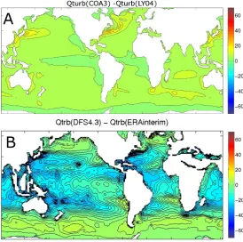
CH,CEandCDare the bulk transfer coefficients for sensi-ble heat, humidity and momentum, respectively. Several pa-rameterizations exist to compute these coefficients. All of them present some uncertainties but the one used in our ocean model NEMO (hereafter LY04) is the one described by Large and Yeager (2004). Even if they are impacted by forc-ing modifications, we chose to focus here on the atmospheric variables corrections, instead of following the approach of Skachko et al. (2009) and Skandrani et al. (2009) used in previous work, because as shown in Fig. 1, the contribution of atmospheric variable error on the net heat-flux uncertainty is more important than the contribution of bulk coefficient uncertainty Brodeau (2007).
2.2 Kalman filtering for parameter estimation
Fig. 1. Top: Mean difference between turbulent heat flux (Qturb=Qlat+Qsens, in W m−2) climatologies (1984–2000) estimated from different bulk algorithms (different transfer coefficients parametrizations): COA3 described by Fairall et al. (2003) and LY04. These clima-tologies are computed with the same atmospheric forcing field and the same prescribed SST (from Brodeau (2007)). Bottom: Mean difference between net heat-flux (in W m−2) climatologies (1989–2007) estimated with air temperature, air humidity and wind speed from different data sets (ERAinterim and DFS4.3 as described in Brodeau et al., 2010). These climatologies only differ by the atmospheric parameters used and are computed with the LY04 bulk algorithm.
the assimilated solution and the forcing. The method de-veloped here proposes an alternative to this classical ap-proach by estimating corrections of a source of model er-rors: the forcing parameters. Here we use the same method-ology (based on a Kalman filter analysis) as developed by Skandrani et al. (2009) to estimate atmospheric forcing pa-rameter corrections. With respect to the classical formulation of the Kalman filter (Kalman, 1960), the control vector ini-tially containing the model state is extended to the forcing parameters that we want to estimate (Eq. 1). The control vec-tor becomes
ˆ
x= x
p
with p=
t2 q2 u10 v10 radsw radlw precip
(1)
withxthe ocean state control vector containing the SST and the SSS, andpthe parameters vector that we aim to correct, wheret2 is the 2 m air temperature,q2 the 2 m air humid-ity,u10the 10 m zonal wind speed,v10the 10 m meridional
wind speed, radswthe downward shortwave radiation, radlw the downward long-wave radiation, and precip the precipita-tion.
The background control vectorxˆfis the model output from a simulation forced by the first guess atmospheric parameters over the assimilation window extended to these atmospheric parameters. We can then obtain the best estimatexˆa of the control vector by taking into account available observations (the vectory):
ˆ
xa=xˆf+ ˆK(y− ˆHxˆf) (2) withxˆfthe background simulation,H the observation opera-ˆ
tor, andK the Kalman gain given byˆ
ˆ
K= ˆPfHˆT(HˆPˆfHˆT+R)−1 (3) with R the observation error, andPˆfthe forecast error covari-ance matrix.
The formulation of the Kalman filter applied to an ex-tended state vector needs to know the forecast error covari-ance matrixPˆfin the augmented space, given by
ˆ
withPˆathe background error covariance matrix, or initialisa-tion error,M the model operator, andˆ Q the model error.ˆ
The knowledge of thePˆfmatrix (and thusPˆaandQ) is cru-ˆ
cial in statistical estimation approaches. As already pointed out by Skachko et al. (2009) the impact of the background error on the model results is even more important when the model state correction is not applied. In their more realistic study, Skandrani et al. (2009) also highlight the fact that mak-ing appropriate assumptions about the forecast error statistics is increasingly important as the problem becomes more real-istic.
However, the objective is here different from these two previous studies, as it focuses on a mean long-term correc-tion of the forcing parameters. The aim is not to correct the model state and improve the short-term forecast of the model, but to estimate long-term atmospheric parameter corrections to be used in another independent free simulation. For this reason, we decided to use a different strategy and to carry out an independent ensemble experiment for each assimila-tion window instead of running a classical chain of analysis cycles. This process simplifies the estimation of the forcing-error covariance matrix (described in Sect. 3). Moreover, un-der the assumption that all the forecast error is due to forcing error and that the forcing correction is ideal, the background error covariance matrix for the next assimilation window is assumed very small. In practice, if we consider that the ini-tialization state of each experiment is close enough to as-similated observations, we can then neglect the initial error covariance error and setPˆa to zero in the expression ofPˆf
(Eq. 4).
The expression of thePˆfmatrix will become ˆ
Pf= ˆQ. (5)
In this approximation, the estimation ofPˆfinvolves only the knowledge of the model error Q generated by forcingˆ
errors during the assimilation window. As this matrix must be representative of forcing parameters errors only, we have to reduce all the other error sources in the ensemble experi-ments to avoid compensation effects in the parameters esti-mation. In this context, the main difficulty is to preserve the robustness of the methodology previously developed. Con-trary to Skachko et al. (2009) and Skandrani et al. (2009), the observation errors need to be taken into account. We do not know the true value of forcing parameters, neither the perfect initial condition that will ensure the efficiency of as-similation experiments. We also have to make the distinction between forcing errors and other potential errors in the sys-tem to obtain the least versatile correction possible. Indeed, the solution will depend on the model used and it could be difficult to apply the same parameter corrections to other con-figurations where the nature of the model error is different. All these matters will be addressed to evaluate the relevance of the method and results in Sect. 4.1.
Finally, two additional refinements of the forecast error statistics will be used in the experiments. First, to avoid spu-rious long range influence of the observations, the ensemble covariance matrix will be localized as described in Brankart et al. (2011), using a horizontal cutting length scale of three grid points (i.e. about 600 km in longitude along the equator). Although it is an arbitrary choice, the length scale of 600 km corresponds to the scale of the impact of a monthly perturba-tion of the forcing. Several possibilities have been tried be-fore choosing this one, which is a good compromise between capturing the impact of a monthly forcing perturbation while not introducing artificial large-scale correlations. Second, to avoid excessive and non-physical parameters corrections, the forecast probability distribution will be assumed to be a trun-cated Gaussian probability distribution, as developed by Lau-vernet et al. (2009), and as already used in Skandrani et al. (2009). In practice, all parameter corrections above 1.5 stan-dard deviations will be truncated.
2.3 Challenge of a realistic application
The first challenge of a realistic application of this method is that available observations of the real ocean are sparse in space and time. We chose to assimilate monthly mean SST data, which is one of the most accurate observations of the ocean, and SSS climatological data to constrain the freshwa-ter budget of the system, and thus to limit unrealistic impact of the correction on the SSS. We use the Hurrel database (Hurrell et al., 2008) giving SST monthly mean between 1989 and 2007, and a climatology of monthly SSS for the same period from Levitus et al. (1998). Since the available information is now more limited than in idealized cases, this application involves some crucial adjustments of the method-ology (see Sect. 3).
The time resolution of available data implies considering assimilation windows of one month, and thus monthly pa-rameters corrections. However we do not have access to the corresponding subsurface mean state to construct the ideal initial condition in order to ensure the validity of the assump-tion ofPˆaequal to zero. For our application, this will be the first adaptation to make to the initial methodology.
With these observations, we will compute corrections to the atmospheric parameters from the ERAi reanalysis avail-able between 1989 and 2007. ERAi is the most recent reanal-ysis produced by the European Center for Meteorological and Weather Forcasting (ECMWF). The atmospheric vari-ables are available every 6 h forXAand every day for XR
and precipitation at the same spatial resolution as the model, but we do not have access to the associated uncertainties. The estimation of the prior probability distribution of the forcing parameters is the second difficulty of a realistic experiment. The monthly uncertainties associated to the parameters have to be characterized. Finally, to run Monte Carlo experiments to estimate the matrixQ, the forcing error in the model hasˆ
3 Error statistics
The forecast error covariance matrixPˆf reflects the impact of the forcing parameters errors on the model state. We esti-mate this matrix by running Monte Carlo experiments, or en-semble experiments, as performed by Skachko et al. (2009) and Skandrani et al. (2009). For each month, we run 200 experiments from the same initial condition. These exper-iments only differ by the atmospheric parameters used to force the model.Pˆf is then deduced from a statistical anal-ysis of the 200 forecast states ensemble. However, to be con-sistent with prior assumptions which are needed to apply the filter methodology, the ensemble experiments have to be rep-resentative of the impact of the forcing parameters error only. We need thus to take care of three constraints that represent the most important methodological developments necessary for a realistic application, and that will be described in the following sections:
– minimization of the model errors that are not due to
the forcing function by a robust diagnostic approach;
– minimization of the initial condition errors;
– computation of parameter perturbations representative
of the forcing uncertainties.
3.1 Robust diagnostic ensemble experiments
The 200 model states ensemble have to be representative of the impact of forcing errors on monthly timescale ocean dy-namics, and particularly on the surface where observations are assimilated. To ensure the consistency of this assumption, other possible errors have to be minimized while performing ensemble experiments. Indeed, the coarse resolution model used here involves parametrization and approximations to compensate unresolved processes. It thus contains errors that are not attributable to forcing, which lead in particular to a bad positioning of the water masses in strong advection re-gions such as western boundary currents. If this type of error is present in the ensemble runs, it will lead to an inconsis-tent estimation of Pˆf, and finally to unphysical parameters compensating the non-forcing errors. As a consequence, en-semble runs have to be as close as possible to the real ocean, and be representative of the forcing errors only.
We chose to constrain the model by using a robust diag-nostic approach (Sarmiento and Bryan, 1982) consisting in a three-dimensional relaxation of the solution to temperature and salinity climatologies (Levitus et al., 1998). Relaxation terms are added to heat, mass and salt conservation equations and create artificial sources and sinks to bring back the sim-ulation to the corresponding climatologies. The relaxation strength is adapted through its time constant. A large value of this time constant corresponds to a light relaxation, and a small one to a strong relaxation. In our case, we adjust the
relaxation time constant to allow the model to react to atmo-spheric forcing without getting to far from the climatology. Two domains are thus specified where the relaxation charac-teristics are different:
– The first 400 m from the surface are likely to be
im-pacted by a forcing modification at monthly timescale. The time constant of the relaxation is one year in this domain to constrain the large-scale feature while al-lowing for a possible impact of the atmospheric fluxes on the dynamics.
– Below 400 m depth, the relaxation applied is strong
with a one-month relaxation constant. The large-scale feature is thus strongly constrained at depth to ensure a good consistency with the observed ocean and limit non-forcing-error sources.
The robust diagnostic approach is a tool used here to pro-duce a density field consistent with an incomplete set of ob-servations. The purpose is to help the identification of a par-ticular set of atmospheric parameters and not to produce a relevant description of ocean circulation. In the constrained simulations, the large-scale water masses positioning in the model solution (e.g. the structure of gyres) are more consis-tent with observed ocean (figure not shown). The first use of the method was to evaluate the ocean response to a given atmospheric CO2 field (Sarmiento and Bryan, 1982). This first approach presents some similarities with our objective to identify the impact on the ocean surface of a given atmo-sphere.
A robust diagnostic simulation introduces artificial sources and sinks of heat and freshwater in the conservation equa-tions and can lead to an unrealistic representation of some processes. However, since the relaxation is lighter in the re-gion directly affected by atmospheric forcing, the relevance of our approach is still valid in this special zone of interest. This three-dimensional relaxation ensures a limited effect of non-forcing errors in the ensemble experiments, so that the
ˆ
Pf matrix is only representative of the errors in the atmo-spheric parameters. The validity of this hypothesis is crucial to estimate consistent parameter corrections and to reduce possible compensation effects.
3.2 Initialization procedure
The second assumption of this study is that the initial error for every month (thePˆa matrix in Eq. 4) can be neglected. IfPˆais non-negligible, then the final equation ofPˆf(Eq. 5) cannot be considered valid. In absolute terms, to ensure that
ˆ
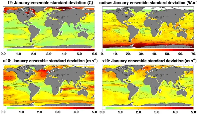
Fig. 2. January ensemble standard deviation in terms of air temperature (top left), shortwave radiation (top right), zonal wind speed (bottom left), and meridional wind speed (bottom right).
simulation we then extract the initial condition that will be used for ensemble experiments. To carry out this simulation, a strong relaxation is applied to the surface in addition to the robust diagnostic approach described in the previous section. The surface relaxation is prescribed with a time constant of two hours to deprive the model of surface evolution freedom. However the objective is to construct an initial condition for the ensemble experiments. This particular initial condition construction is the best compromise that we have found to initialize the ensemble experiments, and it is an important additional procedure allowing a realistic application of the methodology developed by Skandrani et al. (2009) to be car-ried out.
For each month the corresponding initial condition is ex-tracted from the strongly constrained simulation. It is then used to initialize ensemble experiments. To build consistent parameters corrections, the background simulation of one month that gives the background control vector xˆf (Eq. 2) has to be initialized with the same ideal conditions.
3.3 Parameter perturbations computation
The last important assessment to make concerning the en-semble experiments setup is to ensure that the perturbations applied to atmospheric parameters are actually representa-tive of the real forcing uncertainties. It is assumed that pa-rameters uncertainties are comparable to their intra-seasonal and interannual variability in the ERAi reanalysis. This as-sumption turns out to be a fair way to identify parameters uncertainties, but one could envisage other options, such as quantifying the uncertainties by using the local differences between two or more forcing data sets. The parameters prior probability distribution is defined as Gaussian (strictly speak-ing, a truncated Gaussian to avoid extreme parameter
cor-rections, see Sect. 2.2) and its covariance matrix is derived from the ERAi reanalysis intra-seasonal and interannual vari-ability between 1989 and 2007. Perturbations are specific to a given month and constant over each monthly assimilation window. For example, to estimate a set of perturbations for April, we consider the reanalysis signal corresponding to all three month windows (March-April-May) of the reanalysis over the 1989–2007 period (60 states). This Gaussian has a zero mean, and its covariance is defined by the covariance of the parameters around their mean over these three months pe-riods. This assumption is made to characterize the covariance of atmospheric parameters. The choice of intra-seasonal and interannual variability rather than the total variability is made to avoid in the perturbations of April, for example, a variabil-ity that is characteristic of wintertime. A random sample of 200 perturbations is then constructed for each month.
since the ocean model is not involved in the computation of the parameters perturbations. The monthly variability of at-mospheric variables is much larger at high latitudes, particu-larly for the temperature and radiative fluxes, mostly because of the position of the sun influence. The assumption made to generate the parameter perturbations in the ensemble exper-iments could thus be irrelevant in high latitudes regions be-cause changes from one month to another in the three month period can be much larger than the uncertainties. As a conse-quence, the results in these regions must be interpreted cau-tiously. In practice, the whole procedure is repeated monthly between 1989 and 2007, which results in running 200 times the model over the 19 yr period to obtain the set of forcing corrections. Such an important amount of simulations and could be a critical difficulty with a higher resolution model.
4 Results
The objective of this section is to analyze the strength and weaknesses of the methodology that has been adapted to cor-rect ERAi variables. The relevance of specific assumptions described above is evaluated by selecting some diagnostic at global and regional scales. As a first step, we will focus on the capability of the method to isolate the forcing impact in the model and compute realistic parameter corrections. Sec-ond, we will look at the results in terms of global scale heat budget resulting from our corrections. Lastly, we will discuss the impact of the computed corrections in the intertropical band where the method presents the maximum reliability.
4.1 Assessment of the method
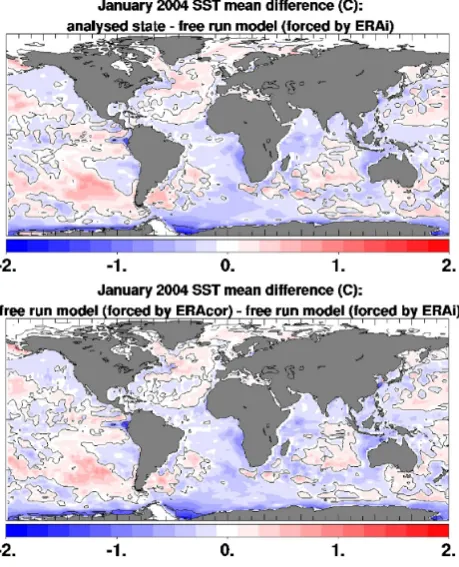
The first important step of the method validation is to look at the results over a specific month (January 2004) which cor-responds to one assimilation window. We compare (Fig. 3, top panel) the SST resulting from the analysis step of the Kalman filter (i.e. the output of Eq. 2), and (Fig. 3, bottom panel) the SST computed by a free model run forced by the newly estimated parameters (hereafter ERAcor). This diag-nostic will determine if the use of corrected parameters in a free simulation has the same impact as the correction com-puted by the analysis scheme. In other words, the objective here is to evaluate if we have properly determined thePˆf
matrix which describes the impact of forcing errors in the model. Figure 3 compares the mean SST increment resulting from the analysis step to the mean SST increment produced in a free run model forced by ERAcor atmospheric variables. In both cases, the resulting SST shows a better agreement with its observed counterpart (not shown). Furthermore, one can see that both increments are very similar in structure and intensity. This result means that the error covariance matrix
ˆ
Pf constructed here is consistent with the actual impact of forcing errors in the model.
Fig. 3. SST differences between the free model run forced by ERAi and the result of the analysis step (top), and between the free model run forced by ERAi and the free model run forced by ERAcor (bot-tom) for January 2004.
The second step to evaluate the reliability of our method to improve the forcing for free model simulations is to look at the consistence of the amplitude of parameter corrections es-timated by the method with the uncertainties on atmospheric variables. Since the focus is here to correct potential long-term trends and mean error, it is of primary importance to as-sess the regional relevance of the corrections temporal mean between 1989 and 2007 (Fig. 4 for the local values, and Fig. 5 for the zonal mean).
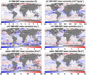
Fig. 4. 1989–2007 mean computed corrections of temperature (t2), humidity (q2), zonal wind speed (u10), meridional wind speed (v10), downward shortwave radiation (radsw), and downward long-wave radiation (radlw).
Fig. 5. 1989–2007 zonal mean computed corrections of temperature (t2), humidity (q2), zonal wind speed (u10), meridional wind speed (v10), downward shortwave radiation (radsw), and downward long-wave radiation (radlw).
mid-latitudes. Long-wave radiation corrections have an op-posite behavior with negative corrections in the intertropical band (−5 W m−2) and positive corrections at mid-latitudes (5 W m−2). The corrections obtained with our method are thus physically reasonable in terms of large-scale intensity and structure.
However, a critical analysis of Fig. 4 allows some per-sisting problems to be identified. These correction fields present some small-scale features (especially at high
Small-scale structures in the Southern Ocean lead to impor-tant gradients in the correction and can result in instability propagation when applied to a free model run. However, crit-ical gradients of 20 to 40 W m−2for the shortwave radiation in this region are not only explained by the localized analysis. Indeed, we noticed in Sect. 3.3 that the assumption made to compute parameters perturbations (and thus parameter prior probability distribution) was not relevant at high latitudes, which can lead to spurious corrections. These spurious cor-rections have obviously not been totally eliminated by the truncation of the prior probability distribution mentioned in Sect. 2. The combination of this problem with the covariance localization hampers the relevance of the correction in the high latitudes.
Figure 4 also allows the results in strong advection re-gions to be looked at more precisely, such as the Gulf Stream, the Kuroshio region, or the Agulhas Current region but also the Antartic Circumpolar Current region. As mentioned in Sect. 3.1, the water masses and front positioning in these regions are not properly represented in our ocean model. Despite of the use of a robust diagnostic approach to com-pute ensemble experiments, these non-forcing errors are still present in the model, with the consequence that estimated corrections in these regions are often excessive (with for example orders of magnitude of 4◦C for the temperature, 3 m s−1 for the zonal wind speed, and up to 60 W m−2 for the shortwave radiation). These values are typical of compen-sation effects. We have here an overestimation of parameter modifications compensating for other model errors. Consid-ering that larger observation errors are not sufficient to by-pass this problem, we cannot be very confident in the realism of estimates made in mid-latitude strong advection regions.
Finally, we observe that the corrections computed for the precipitation field are negligible (figure not shown). This is consistent with the fact that the SSS assimilated aims to avoid unbalanced corrections, and not to actually generate signifi-cant precipitation corrections.
In summary, we have identified in this section the limits of the method implemented to compute upgraded atmospheric variables. And the conclusion is that even if the results look rather consistent with parameter uncertainties in the major part of the world ocean, we have to be cautious with regional corrections computed in the high latitudes and strong advec-tion regions. However these problems remain quite local and we can still look at the global impact of the correction on the ocean heat budget.
4.2 Global results
To study this global impact we have to compute air–sea fluxes corresponding to this new forcing parameters data set using the bulk formulas. The objective here is to evaluate this new data set reliability to force a free model run. The tool used to compute air–sea fluxes offline, using the same formulae as the ocean model and a given atmospheric data
set, was developed by Brodeau (2007). Instead of using the model SST, this diagnostic involves a prescribed SST (here the Hurrel SST). Inter-comparison between different atmo-spheric data set to quantify the parameter modifications im-pact is thus easier than in the model where the SST feedback on the flux computation is taken into account. All fluxes pre-sented in the following are computed using this offline ap-proach. Global results concerning the net heat flux will be presented first, before focusing on the intertropical band to quantify the distribution of this integrated modification over the different net heat-flux components.
The net heat-flux integrates all modifications applied to the latent, sensible and radiative fluxes. The diagnostic of the parameter corrections impact on this flux thus reflects the global effect of forcing modifications. The first criterion used to evaluate a forcing data set is to look at the global heat balance over the considered period (here 1989 to 2007). A balanced budget is a sign of quality for the given forcing. Figure 6 shows that the corrections modify the net heat-flux budget from a positive value of almost 15 W m−2(left) to ap-proximately 2 W m−2(right). This result means that forcing the model with ERAi atmospheric variables would lead to an excessive heating of the ocean, while our corrections re-duce drastically this heat excess and maintain the heat budget close to equilibrium.
Furthermore, a clear negative trend is present in the ERAi time series of the net heat flux. This trend is inconsistent with the observed global warming for the last twenty years (Bindoff et al., 2007). This negative trend is not present any more in the time series of the net heat-flux calculated with the corrected parameters. This diagnostic leads to two crucial results since the methodology does not involve any explicit constraint to obtain a balanced heat budget or to remove po-tential unrealistic trends.
4.3 Intertropical band
Results commented on in Sect. 4.1 allowed regions where reliability of the method is questionable to be identified. To evaluate locally the impact of computed corrections on each net heat-flux component, we chose now to focus on the region between 20◦N and 20◦S, called intertropical band. This region has the advantage not to be affected by spurious corrections or biases in the model circulation mentioned in Sect. 4.1. Furthermore, the model used here has 0.5◦ merid-ional resolution along the equator and thus captures the criti-cal scriti-cales of the equatorial current system (Madec and Im-bard, 1996). As a consequence we expect that the results there reach the maximum reliability. It is thus interesting to go further from the net heat-flux diagnostic and to look at the impact of parameter corrections on the sensible, latent, long-wave radiation and shortwave radiation fluxes.
Fig. 6. 1989–2007 time series of global net heat fluxes monthly means (in red) computed with ERAi variables (left) and ERAcor variables (right). The black lines represent the global mean of the net heat flux over the whole 1989–2007 period.
– temperature and humidity reduced by 0 to 1◦C and 0 to 1 g kg−1, respectively,
– wind speed increased by 0.5 to 1.5 m s−1(Fig. 8),
– downward shortwave radiation increased by 5 to
10 W m−2,
– downward long-wave radiation reduced by 5 to
10 W m−2.
Figure 7 illustrates the impact of these modifications on the mean of the different net heat-flux components over the period 1989–2007. As expected, given the reduced global heat budget, we observe a reduction of the net heat flux of about 20 W m−2. This tends to reduce the warm bias in the intertropical band that can be evidenced by comparing the model SST to the observations (see Fig. 11 described later). Furthermore, since we compute corrections separately for ev-ery atmospheric variable, we can access to valuable informa-tion regarding the relative contribuinforma-tion of each component of the net heat flux to this reduction of the net heat flux. From this diagnostic, it appears that to reduce the heat gain in the intertropical band, the radiative flux (Qsw+Qlw) remains al-most the same (augmentation about 5 W m−2), while the heat loss through turbulent fluxes is clearly increased. As a con-sequence, the net heat flux decrease is mostly due to a mod-ification of the turbulent fluxes. All variable corrections in the intertropical band contribute together to an increased heat loss by turbulent fluxes (decreased temperature and humidity, and increased wind speed).
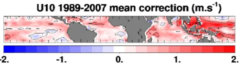
Among these contributions, wind speed is identified by our method to be the essential mechanism involved in the increase of the turbulent heat loss (Fig. 8).
Fig. 8. 1989–2007 mean wind speed correction in the 20◦N–20◦S latitude band. Isocontours from−2 to 2 m s−1by 1.
4.4 Long-term free model simulation
The last diagnostic used here to assess the method is the analysis of a free model run forced by the corrected parame-ters. We showed in the previous sections that our corrections present some unreliable characteristics that could propagate in the model. Parameter corrections are thus post-processed before being used in the model, in order to smooth unrealis-tic small-scale features, and to avoid spurious corrections to be applied in the model.
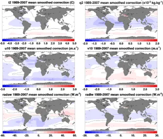
To smooth small-scale features, an anisotropic boxcar fil-ter is applied to each monthly correction. The box size is 10◦ in latitude and 20◦ in longitude in order to keep the zonal signal structure while limiting local gradients. The large-scale correction characteristics thus persist but the parasite structures observed for example in the Southern Ocean are smoothed out as shown in Fig. 9. Since spurious corrections are still present at high latitudes, the corrections are set to 0 for latitudes larger than 60◦in both hemispheres because the error is considered to be mostly due to other processes than forcing (essentially the fact that the method does not take into account the ice cover in these regions). Resulting 1989–2007 mean corrections are shown in Fig. 9.
Although this procedure does not allow the corrections ac-tually computed by the data assimilation method to be tested, the 1989–2007 net heat-flux time series computed from the parameters after correction and from the original ERAi vari-ables are well correlated (>0.5 in the intertropical band), which gives an insight on the good stability of the corrections (e.g., Fig. 10). Furthermore, we can evaluate the corrections in terms of impact in the model focusing on the results in the intertropical band where this post-processing has not a dras-tic impact on the solution since it is the region of correction maximum validity.
In Sect. 4.3 we had shown that the integrated impact of our parameter corrections is to reduce the net heat flux in the in-tertropical band. A reduced SST in the free model run is thus expected when replacing ERAi forcing by corrected parame-ters. In Fig. 11, we first observe that the simulation forced by ERAi variables presents a long-term mean warm bias ranging between 0.5 and 2◦C in the intertropical band (top). Reduc-ing this warm bias to reach values below 0.5◦C for most of the region (consistently with a reduced net heat flux), our cor-rection thus leads to a better agreement with observed SST from a long-term point of view (bottom). Moreover, the
stan-dard deviation of the monthly differences between observed and simulated SST is also reduced by up to 0.2◦C on aver-age in the intertropical band (figure not shown). The strategy developed here to compute independent monthly corrections is thus consistent with our initial objective to improve the long-term mean forcing.
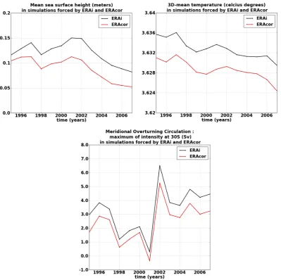
Besides the consistence between observed and simulated SST in the intertropical band, the interannual variability of the model response is not modified by the forcing corrections as shown in Fig. 12. This figure shows the interannual vari-ability of the global means of the SST, the sea surface height (Fig. 12, top panel), and the meridional overturning cell in-tensity at 30◦S (Fig. 12, bottom panel). It is clear that despite the discrepancies between the mean values, the year to year variations are in a very good agreement. This result ensure that the corrections applied do not hampers the interannual variability of the initial ERAi forcing.
5 Conclusions
In this study we explored the feasibility of a sequential data assimilation methodology to estimate monthly corrections of ERAi forcing parameters using real-SST observations. In-dependent monthly data assimilation experiments have been performed over the period 1989–2007 to compute a corrected forcing data set ERAcor (without correcting the model state), to be used in a free model run. The prior probability distri-bution of the parameters has been characterized by the intra-seasonal and interannual variability of ERAi reanalysis, and ensemble experiments of 200 members were performed to estimate the forecast error covariance matrix. Implementing such a methodology in a realistic case is challenging, by the care needed to make assumptions and methodology devel-opments. The initialization procedure of the experiments is crucial to avoid the propagation of potential initial condition errors unrelated to the forcing. For this matter, initial condi-tion as consistent as possible with the surface observacondi-tions has been extracted from a strongly constrained simulation. Moreover, the impact of the forcing on the model state had to be isolated from other model errors in the ensemble experi-ments with a robust diagnostic approach. Finally, the residual excessive corrections have been limited by a truncation of the prior probability distribution of the parameters as described in Skandrani et al. (2009).
This paper illustrates the benefit of using an objective method to estimate forcing corrections. This method has been successfully demonstrated in identifying properly the monthly forcing impact on the model state:
– For every given month, the computed corrections
ap-plied to a free model run have the same impact as the analysis step on the model SST.
– The net heat-flux budget resulting from ERAcor
Fig. 9. 1989–2007 mean corrections of temperature (t2), humidity (q2), zonal wind speed (u10), meridional wind speed (v10), downward shortwave radiation (radsw), and downward long-wave radiation (radlw) after anisotropic boxcar smoothing and masking high latitudes values.
Fig. 10. 1989–2007 ERAi and ERAcor monthlyQnet anomalies time series correlation map. Isocontours from−1 to 1 by 0.2.
global scale, and the potentially unrealistic negative trend observable in the time series of this flux in the ERAi database (leading to ocean cooling) over the whole time period has been removed.
– Parameter corrections computed improve the
long-term mean state of a free (without data assimila-tion) simulation with respect to ocean-surface obser-vations, and can guide typical ad hoc forcing
correc-Fig. 11. 1989–2007 mean differences between Hurrel SST and free model run forced by ERAi (top), and between Hurrel SST and free model run forced by ERAcor (bottom) in the 20◦N–20◦S latitude band.
tions mostly used to adjust forcing parameters (e.g., Brodeau et al., 2010).
Fig. 12. Comparison between the simulations forced by ERAi (black) and ERAcor (red). Top: time series between 1995 and 2007 of the global mean of the sea surface height in m (left), and of the global mean of the temperature in◦C (right). Bottom: time series between 1995 and 2007 of the maximum intensity of the meridional overturning circulation at 30◦S in Sv.
a comprehensive forcing data set including these corrections without introducing any discontinuity in the forcing field be-fore looking at the behavior of the global ocean circulation. However, we diagnosed the equatorial undercurrent in the simulation forced by ERAcor and it turned out that the cor-rected forcing leads to a better representation (in terms of in-tensity) of this important equatorial circulation feature than ERAinterim with respect to TAO observations (not shown). As a further step, one could envisage applying a similar method to an operational system for short term forecast in present-day operational systems. Indeed, the ocean state cor-rection can present some inconsistency with the forcing pa-rameters used, whereas our approach proposes an alternative to keep the interactive ocean–atmosphere link while correct-ing efficiently the ocean surface state.
another model. We could then identify the part of the correc-tion which is dependent to the spatial resolucorrec-tion for example, or to a given formulation used in the model. Unfortunately, this kind of diagnostic would be numerically very expensive, and does not guaranty to capture properly the part of the cor-rection corresponding to the model in all cases but locally in space and time. To go further one could consider to con-strain the water masses by the same type of relaxation but using an ocean reanalysis as reference instead of tempera-ture and salinity climatology. As there are now many atmo-spheric reanalyses available (ERAi, JRA25, NASA MERRA, NCEP/DOE...), the definition of parameter prior probability distribution could also be based on the magnitude differences observed between different atmospheric reanalyses instead of intra-seasonal and interannual variability of a single re-analysis (as in Lucas et al., 2008). This could represent a sub-stantial improvement of the method since it would provide a more realistic description of the parameter uncertainties and would reduce spurious corrections at high latitudes.
Furthermore, the model convergence to assimilated obser-vation strongly depends on the presence of the initialization procedure in the experiments. Parameters computed via this method are thus not necessarily appropriate to reduce the instantaneous discrepancies between model state and obser-vations when applied to a free model long-term simulation. However, our results show that these corrections have a posi-tive impact on the long-term mean values of fluxes and ocean surface state. The heat budget resulting from corrected pa-rameters is closer to zero than the one computed with origi-nal ERAi variables, with a heat excess reduced by more than 10 W m−2. In addition, our corrections remove the unrealis-tic negative trend observed in the time series of the global net heat flux computed with ERAi forcing parameters and the SST of Hurrell et al. (2008). In the intertropical band where we have a maximum validity of the corrections, the warm bias is reduced which leads to a better agreement with surface observations. The diagnostics of the impact on each net heat-flux component allowed the turbulent heat flux to be identified as the main actor of this reduced warming, via wind speed increase in the intertropics essentially. These re-sults are not explicitly prescribed by the method and only result from the ensemble description of the correlations be-tween the forcing variables and the SST.
Several perspectives can now be proposed to go further from this study. On the one hand the method can be im-proved to maximize the impact of observations. In terms of methodology, the first difficulty is that the problem is under-determined: we estimate seven forcing parameters using only two observed variables. This under-determination could be partly reduced by assimilating real SSS observations like SMOS or AQUARIUS when available instead of SSS clima-tology, as well as other ocean profile observations databases like ARGO or TAO. All available observations of the sur-face, the mixed layer or the deep convection regions that are directly influenced by air–sea fluxes would be beneficial to
constrain our system. Recent progresses in intensive ocean observation give a strong potential to our methodology in ad-dressing the problem of the objective computation of forcing correction.
On the other hand further work could be developed in or-der to take advantage of the results already available from our study. Our method is numerically expensive since it involves numerous simulation experiments, and could not reasonably be used at present for higher resolution models. Furthermore, even if the results are inhomogeneous in quality depending on the region considered, the method is certainly able to give valuable insights to guide typical ad hoc forcing adjustments. Results should be first subject to further evaluation by com-parison with available atmospheric or fluxes observations like TAO/TRITON, PIRATA (Pilot Research Moored Array in the Tropical Atlantic), RAMA, and reconstructions based on reanalyses and satellite observations, such as OAflux (Yu and Weller, 2007) or TROPFlux (Praveen Kumar et al., 2011) databases. VOS-based products like NOCS (Berry and Kent, 2009) database can also be useful to conduct further evalu-ation of our correction as far as we consider a region with acceptable sampling error (Gulev et al., 2007). This work would make possible to identify more precisely the strengths and weaknesses of the method, to have a more critical look on the results, and to identify the benefit of the corrections in every particular application.
A wider perspective concerns the implementation of re-analyses. While in the construction of an ocean reanalysis, it is certainly useful to extend the ocean state control vector to the forcing parameters to avoid the propagation of forcing er-rors in the system (e.g., Cerovecki et al., 2011), our method-ology could also be valuable to provide improved ocean boundary information for the implementation of atmospheric reanalyses. Indeed, our approach is not only dedicated to the simulation of the ocean state and can be viewed as an ob-jective way of controlling the air–sea interactions. More pre-cisely, one could envisage to improve boundary conditions in atmospheric models by not using anymore the SST directly but the atmospheric parameters corrections produced by the assimilation of the SST in an ocean model.
Acknowledgements. This research has been conducted with the support of the CNES (French Space Agency) and the CNRS (French National Research center), and received partial support from the EU-funded MyOcean Project (Grant FP7-SPACE-2007-1-CT-218812-MYOCEAN). The calculations were performed using HPC resources from GENCI-IDRIS (Grant 2010-011279).
Edited by: C. Garbe
References
Bindoff, N. L., Willebrand, J., Artale, V., Cazenave, A., Gregory, J. M., Gulev, S., Hanawa, K., Le Quere, C., Levitus, S., Nojiri, Y., Shum, C. K., Talley, L. D., Unnikrishnan, A. S., Josey, S. A., Tamisiea, M., Tsimplis, M., and Woodworth, P.: Observa-tions: oceanic climate change and sea level, In: Climate change 2007: the physical science basis, edited by: Solomon, S., Qin, D., Manning, M., Chen, Z., Marquis, M., Averyt, K. B., Tignor, M., and Miller, H. L., Contribution of Working Group I, Cambridge, Cambridge University Press, 385–428, 2007.
Brankart, J.-M., Cosme, E., Testut, C.-E., Brasseur, P., and Ver-ron, J.: Efficient Local Error Parameterizations for Square Root or Ensemble Kalman Filters: Application to a Basin-Scale Ocean Turbulent Flow, Mon. Weather Rev., 139, 474–493, doi:10.1175/2010MWR3310.1, 2011.
Brodeau, L.: Contribution à l’Amélioration de la Fonction de Forçage des Modèles de Circulation Générale Océanique, Ph.D. thesis, Université Joseph Fourier – Grenoble 1, 2007.
Brodeau, L., Barnier, B., Treguier, A.-M., Penduff, T., and Gulev, S.: An ERA40-based atmospheric forcing for global ocean circulation models, Ocean Model., 31, 88–104, doi:10.1016/j.ocemod.2009.10.005, 2010.
Cerovecki, I., Talley, L., and Mazloff, M.: A comparison of South-ern Ocean air-sea buoyancy flux from an ocean state estimate with five other products, J. Climate, 24, 6283–6306, 2011. Dee, D. P., Uppala, S. M., Simmons, A. J., Berrisford, P., Poli,
P., Kobayashi, S., Andrae, U., Balmaseda, M. A., Balsamo, G., Bauer, P., Bechtold, P., Beljaars, A. C. M., van de Berg, L., Bid-lot, J., Bormann, N., Delsol, C., Dragani, R., Fuentes, M., Geer, A. J., Haimberger, L., Healy, S. B., Hersbach, H., Hólm, E. V., Isaksen, L., Kållberg, P., Köhler, M., Matricardi, M., McNally, A. P., Monge-Sanz, B. M., Morcrette, J.-J., Park, B.-K., Peubey, C., de Rosnay, P., Tavolato, C., Thépaut, J.-N., and Vitart, F.: The ERA-Interim reanalysis: configuration and performance of the data assimilation system, Q. J. Roy. Meteor. Soc., 137, 553–597, doi:10.1002/qj.828, 2011.
Drévillon, M., Bourdallé-Badie, R., Derval, C., Drillet, Y., Lel-louche, J.-M., Rémy, E., Tranchant, B., Benkiran, M., Greiner, E., Guinehut, S., Verbrugge, N., Garric, G., Testut, C.-E., La-borie, M., Nouel, L. Bahurel, P., Bricaud, C., Crosnier, L., Dom-browsky, E., Durand, E., Ferry, N., Hernandez, F., Le Gal-loudec, O., Messal, F., and Parent, L.: The GODAE/Mercator-Ocean global ocean forecasting system: results, applications and prospects, Journal of Operational Oceanography, 1, 51–57, 2008. Fairall, C. W., Bradley, E. F., Hare, J. E., Grachev, A. A., and Edson, J. B.: Bulk Parameterization of Air-Sea Fluxes: Updates and Verification for the COARE Algorithm, J. Climate, 16, 571–591, doi:10.1175/1520-0442(2003)016<0571:BPOASF>2.0.CO;2, 2003.
Ferry, N., Parent, L., Garric, G., Barnier, B., Jourdain, N. C., and the Mercator Ocean team: Mercator Global Eddy Permitting Ocean Reanalysis GLORYS1V1: Description and Results, Mer-cator Ocean Quarterly Newsletter, 36, 15–27, 2010.
Gulev, S., Jung, T., and Ruprecht, E.: Estimation of the Impact of Sampling Errors in the VOS Observations on Air-Sea Fluxes. Part I: Uncertainties in Climate Means, J. Climate, 20, 279–301, doi:10.1175/JCLI4010.1, 2007.
Hurrell, J. W., Hack, J. J., Shea, D., Caron, J. M., and Rosinski, J.: A New Sea Surface Temperature and Sea Ice Boundary Dataset for
the Community Atmosphere Model, J. Climate, 21, 5145–5153, doi:10.1175/2008JCLI2292.1, 2008.
Josey, S.: Air-Sea Fluxes of Heat, Freshwater and Momentum, Op-erational Oceanography in the 21st Century, p. 155, Springer Netherlands, 2011.
Kalman, R. E.: A new approach to linear filter and prediction prob-lems, J. Basic. Eng., 82, 35–45, 1960.
Large, W. and Yeager, S.: Diurnal to decadal global forcing for ocean and sea-ice models: The data sets and flux climatologies, NCAR Tech, Note TN-460+ STR, 2004.
Large, W., Danabasoglu, G., Doney, S., and McWilliams, J.: Sen-sitivity to surface forcing and boundary layer mixing in a global ocean model: Annual-mean climatology, J. Phys. Oceanogr., 27, 2418–2447, 1997.
Lauvernet, C., Brankart, J.-M., Castruccio, F., Broquet, G., Brasseur, P., and Verron, J.: A truncated Gaussian filter for data assimilation with inequality constraints: Application to the hy-drostatic stability condition in ocean models, Ocean Model., 27, 1–17, doi:10.1016/j.ocemod.2008.10.007, 2009.
Levitus, S., Boyer, T., Conkright, M., O’Brien, T., Antonov, J., Stephens, C., Stathoplos, L., Johnson, D., and Gelfeld, R.: World Ocean Database 1998, NOAA Atlas NESDID 18, US Governe-ment Printing Office, Whashingthon, DC, 1998.
Lucas, M. A., Ayoub, N., Barnier, B., Penduff, T., and de Mey, P.: Stochastic study of the temperature response of the upper ocean to uncertainties in the atmospheric forcing in an Atlantic OGCM, Ocean Model., 20, 90–113, doi:10.1016/j.ocemod.2007.07.006, 2008.
Madec, G.: NEMO reference manual, ocean dynamics component : NEMO OPA.Preliminary version, Notes techniques de modéli-sation, Institut Pierre Simon Laplace (IPSL), France, Tech. Rep. 27, ISSN No 1288–1619, 2008.
Madec, G. and Imbard, M.: A global ocean mesh to over-come the North Pole singularity, Clim. Dynam., 12, 381–388, doi:10.1007/BF00211684, 1996.
Milliff, R. F., Large, W. G., Morzel, J., Danabasoglu, G., and Chin, T. M.: Ocean general circulation model sensitivity to forcing from scatterometer winds, J. Geophys. Res., 104, 11337–11358, doi:10.1029/1998JC900045, 1999.
Praveen Kumar, B., Vialard, J., Lengaigne, M., Murty, V., and McPhaden, M.: TropFlux: air-sea fluxes for the global tropi-cal oceans-description and evaluation, Clim. Dynam., 38, 1–23, 2011.
Sarmiento, J. L. and Bryan, K.: An Ocean Transport Model for the North Atlantic, J. Geophys. Res., 87, 394–408, doi:10.1029/JC087iC01p00394, 1982.
Skachko, S., Brankart, J.-M., Castruccio, F., Brasseur, P., and Ver-ron, J.: Improved Turbulent Air-Sea Flux Bulk Parameters for Controlling the Response of the Ocean Mixed Layer: A Sequen-tial Data Assimilation Approach, J. Atmos. Ocean. Tech., 26, 538–555, doi:10.1175/2008JTECHO603.1, 2009.
Skandrani, C., Brankart, J.-M., Ferry, N., Verron, J., Brasseur, P., and Barnier, B.: Controlling atmospheric forcing parame-ters of global ocean models: sequential assimilation of sea sur-face Mercator-Ocean reanalysis data, Ocean Sci., 5, 403–419, doi:10.5194/os-5-403-2009, 2009.
Ves-sel Observations, J. Climate, 14, 4062–4072, doi:10.1175/1520-0442(2001)014<4062:QUINRU>2.0.CO;2, 2001.
Stammer, D., Ueyoshi, K., Kohl, A., Large, W. G., Josey, S. A., and Wunsch, C.: Estimating air-sea fluxes of heat, freshwater, and momentum through global ocean data assimilation, J. Geophys. Res., 109, C05023, doi:10.1029/2003JC002082, 2004.
Sun, B., Yu, L., and Weller, R. A.: Comparisons of Sur-face Meteorology and Turbulent Heat Fluxes over the Atlantic: NWP Model Analyses versus Moored Buoy Observations, J. Climate, 16, 679–695, doi:10.1175/1520-0442(2003)016<0679:COSMAT>2.0.CO;2, 2003.
Wang, W. and McPhaden, M. J.: What is the mean seasonal cycle of surface heat flux in the equatorial Pacific?, J. Geophys. Res., 106, 837–857, doi:10.1029/1999JC000076, 2001.