www.ocean-sci.net/6/331/2010/
© Author(s) 2010. This work is distributed under the Creative Commons Attribution 3.0 License.
Ocean Science
Mediterranean intermediate circulation estimated from Argo data
in 2003–2010
M. Menna and P. M. Poulain
Istituto Nazionale di Oceanografia e di Geofisica Sperimentale – OGS, Sgonico (TS), Italy Received: 20 October 2009 – Published in Ocean Sci. Discuss.: 18 November 2009 Revised: 12 February 2010 – Accepted: 26 February 2010 – Published: 3 March 2010
Abstract. Data from 38 Argo profiling floats are used to describe the intermediate Mediterranean currents for the pe-riod October 2003–January 2010. These floats were pro-grammed to execute 5-day cycles, to drift at a neutral parking depth of 350 m and measure temperature and salinity profiles from either 700 or 2000 m up to the surface. At the end of each cycle the floats remained at the sea surface for about 6 h, enough time to be localised and transmit the data to the Argos satellite system. The Argos positions were used to determine the float surface and intermediate displacements. At the surface, the float motion was approximated by a lin-ear displacement and inertial motion. Intermediate veloc-ities estimates were used to investigate the Mediterranean circulation at 350 m, to compute the pseudo-Eulerian statis-tics and to study the influence of bathymetry on the inter-mediate currents. Maximum speeds, as large as 33 cm/s, were found northeast of the Balearic Islands (western basin) and in the Ierapetra eddy (eastern basin). Typical speeds in the main along-slope currents (Liguro-Provenc¸al-Catalan, Algerian and Libyo-Egyptian Currents) were∼20 cm/s. In the central and western part of Mediterranean basin, the pseudo-Eulerian statistics show typical intermediate circula-tion pathways which can be related to the mocircula-tion of Lev-antine Intermediate Water. In general our results agree with the qualitative intermediate circulation schemes proposed in the literature, except in the southern Ionian where we found westward-flowing intermediate currents. Fluctuating cur-rents appeared to be usually larger than the mean flow. In-termediate currents were found to be essentially parallel to the isobaths over most of the areas characterized by strong bathymetry gradients, in particular, in the vicinity of the con-tinental slopes.
Correspondence to: M. Menna
1 Introduction
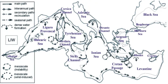
The Mediterranean Sea, depicted in Fig. 1, is a semi-enclosed basin connected to the Atlantic Ocean by the narrow Strait of Gibraltar and to the Black Sea by the Dardanelles-Marmara Sea-Bosphorus system. The whole Mediterranean is a concentration basin (evaporation exceeds precipitation and runoff) divided in two sub-basins (Western and Eastern Mediterranean) by the shallow (∼400 m) sill of the Sicily Channel. The water deficit is supplied by the inflow of the Atlantic Water (AW), that flows from the Strait of Gibral-tar eastward along the North African coast and enters in the eastern basin through the Sicily Channel (Millot, 1999; Las-caratos et al., 1999) (not shown). The net result of the air-sea interactions in the entire Mediterranean is an outflow of salty water through the Strait of Gibraltar; the main water mass that constitute this salty and relatively warm outflow is the Levantine Intermediate Water (LIW). The LIW, formed in the eastern Levantine sub-basin, sinks to a depth between 200 and 500 m and spreads out across the entire Mediterranean basin at this intermediate depth (Fig. 1). The LIW proceeds essentially westward along several pathways and eventually outflows in the Atlantic Sea and influences the formation of North Atlantic Deep Water (NADW) (Reid, 1994; Lozier et al., 1995; Potter and Lozier, 2004). Hence, the salty LIW is a crucial component of the Mediterranean thermohaline “conveyor belt” circulation (Poulain et al., 2007) and it can influence the NADW formation in the global thermohaline cell.
Fig. 1. Circulation of the Levantine Intermediate Water; Mediterranean Sea geography and nomenclature of the major sub-basins and straits
(adapted from Millot and Taupier-Letage, 2005).
mass characteristics (Notarstefano and Poulain, 2009) and currents more or less continuously throughout the Mediter-ranean Sea. We hereafter present a novel quantitative de-scription of the intermediate currents related to the LIW in most areas of the Mediterranean Sea based on the displace-ments of profiling floats.
Autonomous profiling floats were operated in the Mediter-ranean starting in 2000 (Poulain et al., 2007) and contributed to the global Argo program. In 2003, as part of the MF-STEP project, a significant number of floats were deployed to provide temperature and salinity data in real time to op-erational prediction models (http://www.bo.ingv.it/mfstep). These floats, also referred to as MedArgo floats, were pro-grammed to execute 5-day cycles and to drift at a neutral parking depth of 350 m. This depth was chosen because it corresponds approximately to the depth of the LIW core in most of the basin. More specifically a recent study on Argo float salinity data recognizes the LIW core close to the surface in the Levantine basin, at 300–350 m in the centre of Mediterranean Sea and deeper then 350 m in the Liguro-Provenc¸al basin (Notarstefano and Poulain, 2009). Hence, drifts at 350 m allow to study the LIW pathways from its ori-gin in the northern Levantine sub-basin to its outflow through the Strait of Gibraltar (Poulain et al., 2007).
In this paper, we describe quantitatively the Mediterranean Sea circulation at the float parking depth and refer to 350 m currents as intermediate currents. Float surface positions are used to determine surface and intermediate displacements. The estimation of surface displacement includes the use of satellite fixed positions. The estimation of intermediate dis-placement requires the determination of the exact surfacing and diving times and the extrapolation in time of the satellite-derived positions, using a simple model based on linear dis-placement and inertial motion. From these, the intermediate velocities at the 350 m parking depth are estimated and fi-nally used to compute pseudo-Eulerian circulation statistics
and to produce maps of mean intermediate circulation and eddy variability in the Mediterranean Sea.
The paper is organised as follows. Background on the Mediterranean intermediate circulation is given in Sect. 2. The float database and the methodology used to process the data are described in Sect. 3. Fast currents, pseudo-Eulerian maps of mean flow, eddy variability, energy levels and the bathymetry-controlled currents are presented and discussed in Sect. 4. The conclusions are summarized in Sect. 5. Tech-nical details are given in the Appendix A.
2 Background on the Mediterranean intermediate circulation
The most exhaustive descriptions of the intermediate circu-lation in the Western Mediterranean Sea arose in the frame-work of various international projects (La Violette, 1990; Millot, 1995, 1999; Fusco et al., 2003, Millot and Taupier-Letage, 2005), whereas for the Eastern Mediterranean they were described as part of the POEM and MFSPP projects (Malanotte-Rizzoli and Hetch, 1988; Malanotte-Rizzoli and Robinson, 1988; Robinson et al., 1991, 2001; Malanotte-Rizzoli et al., 1999; Fusco et al., 2003). The Mediterranean (Fig. 1) is governed by a large scale anti-estuarine buoyancy-driven circulation (Myers and Haines, 2000): the salinity increase due to evaporation over the Mediterranean surface is compensated by an outflow of salty water in the Atlantic Ocean. Inflowing Atlantic Water (AW) flows across the west-ern and eastwest-ern basins into the Levantine sub-basin. Cooling in winter causes convection to intermediate depths mainly in the Rhodes gyre forming the LIW (Ovchinnikov, 1984; Malanotte-Rizzoli and Robinson, 1988; Lascaratos, 1993; Lascaratos et al., 1993, 1999; Nittis and Lascaratos, 1998; Malanotte-Rizzoli et al., 1999, Myers and Haines, 2000). This salty intermediate water returns to the west underneath
the AW and becomes the main component of Mediterranean outflow to the Atlantic. From Rhodes (Fig. 1), the LIW flows along the southern continental slope of the Cretan Arc is-lands to the Peloponnese, and can be found in the Ierapetra and Pelops wind-induced eddies. Part of the LIW, that con-tinues circulating along the north-eastern slope, penetrates in the Southern Adriatic where it mixes with the AW and in-fluences the deep water formation processes. The remainder bypasses the Southern Adriatic and continues along slope as far as the Sicily Channel, where most of it outflows into the western basin.
Within the Sicily Channel, the LIW flows along the Sicil-ian slope, skirts Sicily and enters in the TyrrhenSicil-ian, where it circulates roughly at 200–600 m. A vein flows out through the Corsica Channel (sill at ∼400 m) while the remainder continues and flows out through the Sardinia Channel. When this vein enters the Algerian sub-basin, part of it can be en-trained offshore by Algerian eddies, the remainder continues along the western Sardinia and Corsica slopes, joins with the vein issued from the Corsica Channel, and enters in the Lig-urian and the Provenc¸al sub-basins. The still-recognisable LIW continues along the Spanish slope (Liguro-Provenc¸al-Catalan Current) and most of it outflows through the Strait of Gibraltar (Millot and Taupier-Letage, 2005). The LIW plays an important role in the functioning of the Mediterranean Sea because it is the warmest and saltiest Mediterranean water formed with large amount, and because it mainly flows along the northern continental slopes of both basins, thus being in-volved in the offshore formation of all deep Mediterranean water (Millot and Taupier-Letage, 2005).
The southern continental slopes of western and eastern basins are characterised by narrow and unstable currents lo-cated respectively in the Algerian (Algerian Current) and Levantine (Libyo-Egyptian Current) sub-basins, that flow from west to east and lead to the generation of cyclonic and anticyclonic eddies (Mejdoub and Millot., 1995; Hamad et al., 2005; Taupier-Letage et al., 2007; Gerin et al., 2009). These currents extend as deep as the LIW core depth (200– 500 m).
During the last decades, direct measurements (moorings) of intermediate currents in some regions of the Mediter-ranean Sea were performed. The results of these in situ ob-servations, summarized below, provide however only a par-tial view of the intermediate flows, with main focus in chan-nels and dominant currents. The intermediate current (300– 400 m) in the northern Tyrrhenian Sea was investigated using three moorings, deployed between 1989 and 1990, that mea-sured velocities values less then 1 cm/s (Artale et al., 1994). One year of current measurement in the Corsica Channel (be-tween October 1986 and September 1987), obtained from three moorings deployed in the area north of Corsica and off the eastern Ligurian coast, produced respectively a mean velocity of 8.4 , 5.6 and ∼10 cm/s at depth of 300 m (As-traldi et al., 1990). An array of nine moorings, deployed in the eastern Algerian Basin between July 1997 and July 1998,
measured a mean current of 4.8 cm/s and a maximum current of 14.73 cm/s (Testor et al., 2005). Two years (1994–1995) of direct current measurements were collected by six moor-ings in the Otranto Channel; in the intermediate layer (290– 330 m), speed showed the minimum values in the central re-gion of the channel (between 0.3 and 0.8 cm/s), maximum value along the eastern boundary (4.4 cm/s) and a mean value of 1.3 cm/s at the western boundary (Kovaˇcevi´c et al., 1999). In the same period, moorings located in the southern Adriatic recorded mean velocities between 1.4 and 5 cm/s (Kovaˇcevi´c et al., 1999). In the Sicily Channel, over the western sill of the strait, the outflow of Eastern Mediterranean intermediate water was characterised by an intensity of 12.5 cm/s, whereas at the southern entrance of the Tyrrhenian Sea the intermedi-ate current showed a speed of∼8 cm/s (Astraldi et al., 2001). In summary, we can state that the intermediate speeds mea-sured by moorings in the Mediterranean Sea vary essentially between 1 and 15 cm/s.
3 Data and methods
3.1 Float data
Two types of profiling floats were operated in Mediter-ranean: the Apex (manufactured by Webb Research Corpo-ration, USA) and the Provor (produced by NKE Electronics, France). All floats were equipped with Sea-Bird CTD sen-sors.
Among all the floats deployed in the Mediterranean Sea, we have selected 38 instruments according to their cycle characteristics. They were deployed as part of the MFSTEP project in 2003 and are referred to as MedArgo floats. Each float descents from the surface to a programmed parking depth of 350 m, where it remains for about 4.5 days before reaching the profile depth, that is generally 700 m but ex-tends to 2000 m every ten cycles. At the end of each cycle the float remains for about 5–7 h at the sea surface (Solari et al., 2008), where it is localised by, and transmit the data to, the Argos satellite system. Argos is a global data loca-tion and collecloca-tion system carried by the NOAA polar orbit-ing satellites; this system provides the float positions with an accuracy between 250 and 1500 m (see Appendix A for details). The data used in this work contain information on three dimensional movement of float: a set of coordinates of the float during its transmissions from the sea surface to the satellites and the pressure recorded during the parked phase of the cycle. These data are utilized to determine the float surface and intermediate displacements and, consequently to estimate the parking depth velocities.
Fig. 2. Trajectories of the MedArgo floats between October 2003 and January 2010. Black lines represent surface and intermediate raw
trajectory (obtained by 3431 cycles) filtered to remove cycles located over depths less then 350 m and anomalous cycles larger than 5 days. Colored segments depict intermediate displacement (obtained by 2963 cycles); each color represents a different velocity range. The 200 and 2000 m isobaths are shown with grey curves.
October 2003 and January 2010. Colored segments empha-size intermediate displacements obtained with the method explained hereafter; they correspond to 2963 floats cycles. The best sampled regions are located in the western and east-ern basins, whereas the central regions of Mediterranean Sea (Adriatic, Sicily Channel) and the Aegean Sea are less or not sampled.
3.2 Data processing
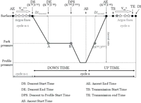
The schematic diagram in Fig. 3 shows in detail a float cy-cle and two subsequent float transmissions. The stars rep-resent satellite received positions (fixes). The deep currents can be estimated by dividing the distance that floats move at the parking depth (displacement between A and B), by the duration of drift (time interval between DE – Descent End Time and DPS – Descent to Profile Start Time), which re-quires knowledge of the time and position of diving (DS – Descent Start Time; (XDS, YDS))and surfacing (AE – As-cent End Time; (XAE, YAE)); this critical information is not directly measured by floats (Park et al., 2004, 2005).
In first approximation, the intermediate velocities (Vold) are estimated using the last position of cyclen−1 and the first position of cyclen(grey stars in Fig. 3), according to Lebedev et al. (2007). The drawback of this method is that the unknown drift, while floats are at the surface (before the first and after the last fix), generates a significant source of er-ror in estimating the deep current, because currents are much stronger at and close to the surface than at the parking depth. To improve the first approximation results, we estimated the best float surface displacements (second approxima-tion) according to the method of Park et al. (2005) (see Appendix A). This involves the estimation of diving (DS; (XDS, YDS))and surfacing (AE;(XAE, YAE))times and po-sitions and of their errors. The intermediate displacement is
Fig. 3. Schematic diagram of depth versus time of a float cycle and
two subsequent float transmissions.
considered as the distance between the position(XDS, YDS) at cyclen−1 and the position(XAE, YAE)at cyclen. The diving and surfacing times and positions are used to estimate the intermediate currents (V350).
The comparison between rough (1st approximation – Vold)and fine (2nd approximation –V350)estimates of inter-mediate current near 350 m, suggest to select, for the pseudo-Eulerian calculation statistics, an intermediate current dataset (Vend350)composed of all consecutive cycles with surface skill in excess of 0.8 (for definition of skill see Appendix A). Af-ter this selection the number of velocity estimates (Vend350)is 2963.
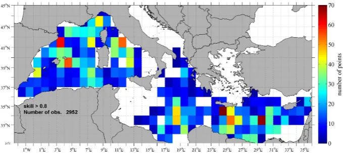
Fig. 4. Spatial distribution of the float intermediate velocity observations in 1◦×1◦bins.
3.3 Pseudo-Eulerian statistics
Lagrangian velocity data (Vend350), derived from floats dis-placements at 350 m, are used to estimate Mediterranean mean intermediate circulation field. The mean flow recon-struction is performed through the “pseudo-Eulerian” aver-aging, using about six years (October 2003–January 2010) of float intermediate velocities, spatially averaged in boxes of 1◦×1◦. Figure 4 shows the data density inside the boxes. The bins with high number (>30) of observations are lo-cated in some areas of the western region (Tyrrhenian Sea and Liguro-Provenc¸al sub-basins), in the eastern region (Lev-antine sub-basin) and in proximity of the Libyan coast. Bins with only one observation are rejected. Mean velocity vec-tors, mean standard error, velocity variance ellipses, kinetic energy of the mean flow per unit mass (MKE – mean kinetic energy), and mean eddy kinetic energy per unit mass (EKE – eddy kinetic energy) are calculated from the 1◦×1◦binned floats data, according to Poulain et al. (2001). In some re-gions of Mediterranean Sea, characterised by sub-basin and mesoscale structure (eddies with a maximum diameter of ∼100 km), the float velocities are spatially mapped with a higher bin resolution (0.5◦×0.5◦).
3.4 Bathymetry
In order to evaluate the influence of the bathymetry on the intermediate Mediterranean currents, we used the Smith and Sandwell Bathymetry (Smith and Sandwell, 1997) Model topo 8.2.img, a 2-min (about 4 km) Mercator-projected grid, based on bathymetry derived from satellite gravity data com-bined with ship measurements. The north and east gradient components, interpolated at the positions corresponding to theVend350 dataset, are used to evaluate the across and along bathymetry components of the float velocity.
4 Results
4.1 Fast currents
Intermediate displacements collected in theVend350dataset are shown with colored segments in Fig. 2; each color repre-sents a different velocity range. Maximum speeds as large as 33 cm/s are found northeast of Balearic Islands and in the Ierapetra eddy. Speeds larger than 20 cm/s are reached in the north and central regions of Liguro-Provenc¸al-Catalan sub-basin and in some eddies of the eastern sub-basin. The Liguro-Provenc¸al, Algerian and Libyan-Egyptian Currents are char-acterised by maximum speeds of 15 cm/s.
4.2 Pseudo-Eulerian statistics
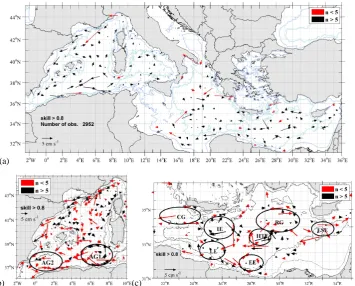
Figure 5a shows the Mediterranean pseudo-Eulerian mean circulation field, derived from 1◦×1◦binned float velocities dataVend350). Figure 5b and c shows the pseudo-Eulerian maps with higher bin resolution (0.5◦×0.5◦) to emphasize some dynamical structures with a spatial scale less then 100 km. In each bin, the mean velocity vector is positioned in the center of mass of the observations. The standard error of bin-averaged velocities was calculated using the degrees of freedom in each bin equal to the number of observations. The mean value of the standard error is 0.7 cm/s and its maximum value is 3.9 cm/s, achieved in a bin with less than 5 observa-tions.
(a)
(b) (c)
Fig. 5. (a) Pseudo-Eulerian mean circulation field at 350 m, derived from 1◦×1◦binned floats velocities data (Vend350). (b) Detail of the Western Mediterranean basin (bins of 0.5◦×0.5◦) and location of the Algerian Gyres (AG1, AG2). (c) Detail of the Eastern Mediterranean basin (bins of 0.5◦×0.5◦) and location of the main sub-basin eddies and gyres: Cretan Gyre (CG), Ierapetra Eddy (IE), Egyptian Eddy (EE), Libyan Eddies (LE), Herodotus Trough Eddy (HTE), Rhodes Gyre (RG), Eratosthenes Seamount Eddy (ESE).
with a mean velocity of 2 cm/s (MKE less than 10 cm2/s2, Fig. 7a), following the western coasts of Sardinia and Cor-sica, while another branch proceeds to the west (bin-averaged speed between 3 and 7 cm/s, Fig. 5b; MKE between 10 and 25 cm2/s2, Fig. 7a) and enters the Algerian Basin.
In the Liguro-Provenc¸al sub-basin intermediate mean ve-locities describe a cyclonic circulation that, according to As-traldi et al. (1994), typically involves both the surface and the intermediate layer; in this region LIW participates with surface Atlantic Water (AW) in the wintertime formation of West Mediterranean Intermediate Water (WIW) (Robinson et al., 2001). The float velocities vary between 3 cm/s in the eastern branch (in agreement with Astraldi et al., 1994) and 11 cm/s in the western branch. The main cyclonic path (41◦–44◦N; 0◦–8◦E) contains a re-circulation cyclonic
cell located between 42◦–44◦N and 6◦300–8◦300E (Fig. 5b).
Along the French and Spanish slopes, the float veloci-ties follow the Liguro-Provenc¸al-Catalan Current (or North-ern Current), and reach the maximum bin-averaged speed (∼11 cm/s) and the maximum value of MKE (∼65 cm2/s2, Fig. 7a) recorded in the float dataset. In the Balearic Sea, around the islands of Majorca and Menorca, the intermediate mean current describe an anticyclonic circulation following the isobaths; south of the Ibiza Channel the current merges
into the Liguro-Provenc¸al-Catalan flow, towards the Albor´an Sea. In the Algerian Basin the floats follow the Algerian Cur-rent along the coast from west to east, with a maximum ve-locity of∼7 cm/s (Fig. 5a and b) and MKE values between 15 and 30 cm2/s2(Fig. 7a). More offshore they describe two cyclonic gyres (AG1 and AG2 in Fig. 5b), defined as Eastern Algerian and Western Algerian Gyres (Testor et al., 2005; Testor and Gascard, 2005) with a geographical extension of 100–300. The water masses recognised in AG1 and AG2 are composed by highly modified LIW and Tyrrhenian Deep Wa-ter (TDW). The mean float velocities in the Algerian Gyres at 350 m are in agreement with Testor et al. (2005) results (mean value∼5 cm/s; maximum value∼10 cm/s).
In the southern Ionian Sea, the float velocities show a dominant anticyclonic circulation between 32◦–36◦N and
16◦–20.5◦E, in which the southern limb corresponds to a
north-westward flow located on the African continental slope (speeds between 1.5 and 9 cm/s, Fig. 5a; MKE values be-tween 10 and 40 cm2/s2, Fig. 7a).This north-westward cur-rent is in opposite direction compared to the circulation pat-terns described by Millot and Taupier-Letage (2005) and de-picted in Fig. 1. In the south of Levantine Basin (Fig. 5c), along the Libyan and Egyptian slopes, the mean currents flow eastward and turn into several eddies, progressing
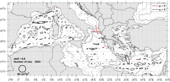
Fig. 6. Velocity variance ellipses at 350 m obtained from 1◦×1◦binned floats velocity field.
downstream along the slope (Libyan Eddy-LE and Egyptian Eddy-EE). In the Cretan Passage the vectors follow the Ier-apetra anticyclonic Eddy (IE). More to the east it is possible to recognize the Herodotus Trough anticyclonic Eddy (HTE), documented by Gerin et al. (2009) and Taupier-Letage et al. (2007). Moreover, the float intermediate mean circulation describes the Rhodes cyclonic Gyre (RG) to the north and, south of Cyprus Island, the anticyclonic eddy that sits over the Eratosthenes Seamount (Eratosthenes Seamount Eddy-ESE). All the Levantine basin is characterised by MKE val-ues less than 20 cm2/s2(Fig. 7a) and maximum velocity of ∼7 cm/s (Fig. 5a and c).
Figure 6 shows the velocity variance ellipses at 350 m. The maximum value (64 cm2/s2, rms speed∼8 cm/s) is reached in the North Balearic Thermal Front area, which represents a transition region between two different dynamic regimes (Garc´ıa et al., 1994). High values (60 cm2/s2, rms speed ∼9 cm/s) are also reached in the eastern basin around Crete Island, in the Ierapetra Eddy area. The velocity variance is typically oriented in the direction of the mean currents. In the coastal or along-slope currents such as the Algerian and Liguro-Provenc¸al-Catalan Currents, the major axes of the ve-locity variance ellipses are parallel to the coastline. In the open sea, the ellipses are generally less elongated but pre-dominantly oriented in the zonal direction. The mean ki-netic energy of fluctuating velocity, EKE, follows the vari-ance field and reaches values as large as 60–80 cm2/s2in the centre of the Levantine Basin and in the Liguro-Provenc¸al re-gion (Fig. 7b). EKE has strong gradients compared to MKE; the ratio of EKE to MKE (not shown) provides information on the energy distribution between mean constant and fluctu-ating currents in the Mediterranean Sea. In general, the EKE value is larger than MKE (ratio>1) except in some coastal regions characterised by permanent currents. This result sug-gests that the energy of intermediate currents is dominated by the velocity fluctuating component.
4.3 Bathymetry effect
338 M. Menna and P. M. Poulain: Mediterranean intermediate circulation
(a)
(b)
8 M. Menna and P. M. Poulain: Mediterranean intermediate circulation
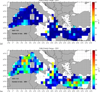
Fig. 7. Energy distribution between mean constant (a) and fluctuating (b) currents in the Mediterranean Sea.
5 Conclusions
The trajectories of 38 Argo floats, deployed in the Mediter-ranean Sea between October 2003 and January 2010, are used to create a dataset of velocities at 350 m and to study the intermediate circulation in regions with good data cov-erage (Western Mediterranean, Ionian and Levantine sub-basins and Cretan Passage).
The velocity dataset is produced through three different steps: the first provides rough estimates of intermediate ve-locities (Vold), according to Lebedev et al. (2007); the sec-ond produces the best surface velocities according to Park et al. (2005); the third provides the intermediate displacement (V350)that involves the use of the diving and surfacing times and positions. From the comparison betweenVoldandV350 and the results of the statistical analysis computed onV350, we select only the best estimates of velocities (variance ex-plained/total variance>0.8) to produce the final datasetVend350. The amplitude of the Vend350 velocities reach the maxi-mum values of ∼33 cm/s east of the Balearic Islands and in the Ierapetra eddy; high speeds (larger than 20 cm/s) are also found in the north and central regions of the
Liguro-Provenc¸al-Catalan basin and in some eddies of the eastern basin, whereas the Liguro-Provenc¸al, Algerian and Libyan-Egyptian Currents are characterised by maximum speeds of 15 cm/s.
The pseudo-Eulerian statistics, computed withVend350, show typical circulation pathways related to Mediterranean inter-mediate currents. The mean circulation mapped by floats is almost everywhere in agreement with the description of inter-mediate circulation provided by the framework of various in-ternational projects and by several authors in the past. There is an important exception in the southern Ionian, along the Libyan coast, where floats follow a north westward current, which is in opposite direction compared to the circulation patterns described by Millot and Taupier-Letage (2005) and depicted in Fig. 1. The LIW flow south of Crete and north-ward pathway tonorth-ward the Adriatic Sea was not confirmed by the float data, due to the presence of Ierapetra eddy and the scarcity of data in the northeast Ionian Sea.
In the Western Mediterranean basin, the velocity field shows the characteristic cyclonic paths in the Tyrrhenian, Liguro-Provenc¸al and Algerian sub-basins, as well as in the Algerian and Liguro-Provenc¸al-Catalan Currents, where it
Ocean Sci., 6, 1–13, 2010 www.ocean-sci.net/6/1/2010/ Fig. 7. Energy distribution between mean constant (a) and fluctuating (b) currents in the Mediterranean Sea.
5 Conclusions
The trajectories of 38 Argo floats, deployed in the Mediter-ranean Sea between October 2003 and January 2010, are used to create a dataset of velocities at 350 m and to study the intermediate circulation in regions with good data cov-erage (Western Mediterranean, Ionian and Levantine sub-basins and Cretan Passage).
The velocity dataset is produced through three different steps: the first provides rough estimates of intermediate ve-locities (Vold), according to Lebedev et al. (2007); the sec-ond produces the best surface velocities according to Park et al. (2005); the third provides the intermediate displacement (V350)that involves the use of the diving and surfacing times and positions. From the comparison betweenVoldandV350 and the results of the statistical analysis computed onV350, we select only the best estimates of velocities (variance ex-plained/total variance>0.8) to produce the final datasetVend350. The amplitude of the Vend350 velocities reach the maxi-mum values of ∼33 cm/s east of the Balearic Islands and in the Ierapetra eddy; high speeds (larger than 20 cm/s) are also found in the north and central regions of the Liguro-Provenc¸al-Catalan basin and in some eddies of the eastern
basin, whereas the Liguro-Provenc¸al, Algerian and Libyan-Egyptian Currents are characterised by maximum speeds of 15 cm/s.
The pseudo-Eulerian statistics, computed withVend350, show typical circulation pathways related to Mediterranean inter-mediate currents. The mean circulation mapped by floats is almost everywhere in agreement with the description of inter-mediate circulation provided by the framework of various in-ternational projects and by several authors in the past. There is an important exception in the southern Ionian, along the Libyan coast, where floats follow a north westward current, which is in opposite direction compared to the circulation patterns described by Millot and Taupier-Letage (2005) and depicted in Fig. 1. The LIW flow south of Crete and north-ward pathway tonorth-ward the Adriatic Sea was not confirmed by the float data, due to the presence of Ierapetra eddy and the scarcity of data in the northeast Ionian Sea.
In the Western Mediterranean basin, the velocity field shows the characteristic cyclonic paths in the Tyrrhenian, Liguro-Provenc¸al and Algerian sub-basins, as well as in the Algerian and Liguro-Provenc¸al-Catalan Currents, where it reaches the maximum intensities (∼10–12 cm/s). High val-ues of EKE (∼80 cm2/s2)and velocity variance are reached
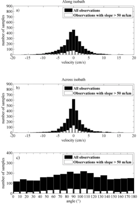
Fig. 8. Histograms of along-isobath (a) and across-isobath (b)
com-ponents of the currents and their directions (c) with respect to the bathymetry gradients. All the observations are depicted in black; those located on significant slope are depicted in white.
in the North Balearic Thermal Front area; the velocity vari-ance is oriented in the direction of mean currents. In the eastern basin the mesoscale and sub-basin scale circulation is dominated by eddies, with the maximum value of EKE (∼60 cm2/s2)and variance located south of Crete (Ierapetra eddy). All over the Mediterranean Sea the EKE has strong gradients compared to MKE. The MKE (maximum value ∼60 cm2/s2)dominates the energy of intermediate currents only in a few regions, characterised by high velocity fields (Liguro- Provenc¸al-Catalan and Algerian Currents, centre of Ionian Sea), whereas it is less then 20 cm2/s2in most of the open sea.
In the regions with significant bathymetry gradients, that is mostly along the continental shelf slope, intermediate cur-rents are driven by topography and the along-isobath compo-nents of velocity have values larger than the across-isobath components. Speeds have mean values of∼5 cm/s and reach 20 cm/s east of Balearic Islands, in the Cretan Passage and in the southern entrance of Tyrrhenian Sea.
Fig. A1. Example of extrapolation results. The solid line
repre-sents the satellite fixed trajectory; small circles and triangles show the intermediate and extreme fixed positions respectively; the big circles are representative of the position quality class. The dashed line represents the extrapolated trajectory and stars the extrapolated positions; diamonds and squares depict DS and AE extrapolated po-sitions, respectively.
The displacements of Argo floats at 350 m depth in the Mediterranean, processed with the methods exposed in this paper, provide a novel quantitative description of the inter-mediate Mediterranean currents, partially related to the path-ways of the LIW. This description confirms, contradicts (in the southern Ionian) and expands the results of previous qual-itative studies, mostly based on hydrographic, satellite and mooring data. It is hoped that the continuation of the Argo program in the Mediterranean with the standard parameters (cycles of 5 days, parking depth near 350 m) will provide more abundant data in the whole Mediterranean Sea in order to improve the results presented in this paper, and eventually monitor long-term changes in the mean intermediate circula-tion related to climate change.
Appendix A
A1 Float surface displacement
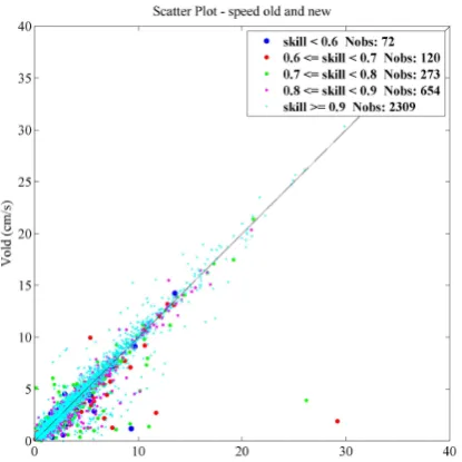
Fig. A2. Scatter plot ofVoldversusV350; colours correspond to
different classes of skill.
(Fig. 3), according to the instructions contained in the Apex-Profiler User Manual.
To determine the surfacing and diving positions, it is nec-essary to extrapolate the surface trajectory determined from discrete Argos satellite fixes (Davis et al., 1992; Park et al., 2004, 2005; Davis, 2005). According to the extrapolation method of Park at al. (2005), we assume that a float sur-face trajectory is the sum of a linear drift, inertial motion and noise. Hence, the extrapolated positions(xk,yk)at the timetkcan be written as:
xk=ul1t+(x0−xi)cos(−f 1tk)
−(y0−yi)sin(−f 1tk)+x (A1) yk=Vl1t+(x0−xi)sin(−f 1tk)+(y0−yi)sin(−f 1tk)
+yi
1tk=tk−t0,(k=0,...N−1) (A2) whereNis the number of data fixes,(x0,y0)are the reference positions at timet0,(xi,yi)represent the centre of the inertial motion,(ul,Vl)are the components of linear velocity andf is the inertial frequency. There are 6 unknown parameters required to reproduce a float trajectory; all these parameters (ul,Vl,x0,y0,xi,yi)are obtained using a least square linear model to minimize the cost function:
J= N X
k
(xk−xobs)2+(yk−yobs)2 2σk2
; (A3)
where(xobs,yobs)are the observed positions andσkthe stan-dard deviations (quality) of the observed positions (Argos satellite system has three different classes of quality for the determination of instrument position: class 1, 2 and 3 with accuracy of 1500 m, 500 m, 250 m, respectively).
Table A1. Statistical parameters related to the cycle 142 of Provor
float b35506. Inertial period, Surface time (time that float spent at sea surface), Time after (time interval between the arrive of float at sea surface and the first transmission received by the satellite), Time before (time interval between the last transmission received by the satellite and the immersion of float), number of Argos posi-tions, Cost function (differences between extrapolated and observed position divided by standard deviation), Skill (see Appendix A for details),(uobs,Vobs)(velocities computed from the last and first
po-sitions),(uex,Vex)(velocities computed from diving and surfacing
positions),Vinertial(inertial velocity), Inertial radius.
Float b35506 cycle 142 Inertial period (h) 17.20 Surface time (h) 7.47 Time after (h) 0.13 Time before (h) 2.22 Argos positions 9 Cost function 0.03 Skill 0.97
uobs(cm/s) −36.47 vobs(cm/s) 11.04 uex(cm/s) −35.25 Vex(cm/s) 14.44 Vinertial(cm/s) 1.69 Inertial radius (km) 0.17
Table A2. Extrapolated positions errors versus skill.
Number of cycles Explained Varince Error (km) available for test 0.5≤Skill<0.6 2.41 79 0.6≤Skill<0.7 1.97 112 0.7≤Skill<0.8 1.33 180 0.8≤Skill<0.9 1.21 425 0.9≤Skill<1 1.19 1838
Figure A1 shows an example of results of this model, called linear-inertial model, for cycle 142 of float b35506. The satellite-fixed trajectory is traced by a solid line; the cir-cles and triangles on the line represent the intermediate and extreme fixed positions of the cycle, respectively; each po-sition is at the centre of a circle representative of the posi-tion quality class. The extrapolated linear-inertial trajectory is traced by a dashed line, with stars representing the extrap-olated positions, whereas diamonds and squares depict DS and AE extrapolated positions, respectively.
The statistics related to the cycle in Fig. A1 are reported in Table A1. The most interesting parameters are the cost function valueJ, which show the differences between the ex-trapolated and observed positions, and the value of explained variance, also called skill or coefficient of determination,R2.
Table A3. Statistical results related to the cycles with skill higher then 0.6.
Explained Number of mean (V350−Vold) Standard Correlation Varince observations (cm/s) Deviation (cm/s) Coefficent Skill≥0.6 3356 0.12 5.21 0.88 Skill≥0.7 3236 0.10 5.23 0.90 Skill≥0.8 2962 0.08 5.28 0.93 Skill≥0.9 2309 0.04 5.44 0.93
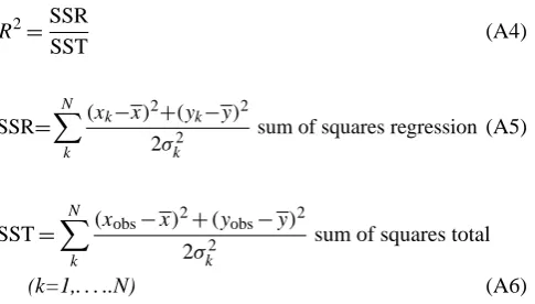
The skill is a statistical parameter that identifies the effective-ness of a model to estimate the observed trajectories: R2=SSR
SST (A4)
SSR= N X
k
(xk−x)2+(yk−y)2
2σk2 sum of squares regression (A5)
SST= N X
k
(xobs−x)2+(yobs−y)2
2σk2 sum of squares total
(k=1,. . . ..N) (A6)
Here, SST is the variance in the data and SSR is the amount of variance explained by our regression model. If the regres-sion curve fits perfectly all the sampled values, all residuals should be zero and SSR/SST=R2=1; as the fit becomes in-creasingly less representative of the data points,R2decreases toward a possible minimum of zero (Emery and Thomson, 2007). In some cycles the linear-inertial model tend to overestimate the inertial component of velocity (results not shown). In these situations, the skill related to simple lin-ear regression model (straight line) is higher then the one of the combined linear-inertial model. In order to minimize this source of error we selected, for each cycle, the best approx-imation between the linear and linear-inertial models. The results are used to determine surfacing and diving positions and the related float surface velocity(uex,Vex).
A2 Estimation of errors
The accuracy of extrapolation method is estimated using the observed positions. The first and last fixes of each cycle are removed and the extrapolation procedure applied, to calcu-late these positions from the remaining observations (Park et al. 2004). To perform the test only cycles with more then 5 observed positions are selected and divided in differ-ent classes according to their skill interval. In each class the differences between extrapolated and fixed extreme positions are evaluated. The mean error, summarized in Table A2, de-creases when the skill inde-creases. The best result is∼1.2 km, obtained with skills major then 0.8.
To improve the estimation of intermediate displacement, we evaluated the arrival (DE) and departure (DPS) times and relative positions (XDE, YDE)(XDPS, YDPS) at park-ing depth (Menna and Poulain, 2009) through the ap-plication of a vertical linear velocity shear. The mean difference between surfacing (XAE, YAE) and diving (XDS, YDS)extrapolated positions and the respective posi-tions((XDPS, YDPS);(XDE, YDE))at 350 m (∼3 km) have the same order of magnitude of the error between extrapo-lated and observed positions. We concluded that the appli-cation of shear actually represents an additional source of error, and decided to not take it into account explicitly and to calculate the velocity vectors (V350)between the diving positions(XDS, YDS)at cyclen−1 and surfacing positions (XAE, YAE)at cyclen. Considering both the extrapolation errors at the surface and the float displacements during de-scent and ade-scent, we estimated an error of about 1 cm/s on the intermediate velocities, using a time interval of about 4.5 days.
A3 Comparison between rough (1st approximation) and fine (2nd approximation) estimates of intermediate current near 350 m
Each velocity dataset at 350 m (V350), obtained in second approximation, is compared with the first approximation ve-locity (Vold). The scatter plot in Fig. A2 reveals a large pos-itive correlation between the two variables; colours display different classes of skill.
Table A3 shows the statistical results related to the cycles with skill higher then 0.6. For skill≥0.8 the mean difference is negligible, the standard deviation is<5.3 cm/s and corre-lation coefficient is 0.93. From these results we decided to consider, for the computation of pseudo-Eulerian statistics, a dataset (Vend350)composed by all consecutive cycles with sur-face skill major then 0.8.
Acknowledgements. This work was co-funded by the European
Thanks to R. Gerin, G. Notarstefano, A. Bussani and G. Bolzon for their help with the data processing and stimulating discussions. The anonymous referees are acknowledged for their constructive comments.
Edited by: S. Josey
References
Artale, V., Astraldi, M., Buffoni, G., and Gasparini, G. P.: Seasonal variability of gyre-scale circulation in the northern Tyrrhenian Sea, J. Geophys. Res., 99(C7), 14127–14137, 1994.
Astraldi, M. and Gasparini, G. P.: The Seasonal Characteristic of the Circulation in the Tyrrhenian Sea, Coast. Estuar. Stud., 46, 115–134, 1994.
Astraldi, M., Gasparini, G. P., Gervasio, L., and Salusti, E.: Dense water dynamics along the Strait of Sicily (Mediterranean Sea), J. Phys. Oceanogr., 31, 3457–3475, 2001.
Astraldi, M., Gasparini, G. P., Manzella, G. M. R., and Hopkins, T. S.: Temporal Variability of Currents in the Eastern Ligurian Sea, J. Geophys. Res., 95(C2), 1515–1522, 1990.
Astraldi, M., Gasparini, G. P., and Sparnocchia S.: The Sea-sonal and Interannual Variability in the Ligurian-Provenal Basin, Coast. Estuar. Stud., 46, 93–113, 1994.
Davis, R.: Intermediate-Depth Circulation of the Indian and South Pacific Oceans Measured by Autonomous Floats, J. Phys. Oceanogr., 35(5), 683–707, 2005.
Davis, R., Webb, L., Regier, L., and Dufour, J.: The Autonomous Lagrangian Circulation Explorer (ALACE), J. Atmos. Ocean. Tech., 9, 264–285, 1992.
Emery, W. J. and Thomson R. E.: Data Analysis Methods in Physi-cal Oceanography, Elsevier, Amsterdam, 638 pp., 2007. Fusco, G., Manzella, G. M. R., Cruzado, A., Gacic, M.,
Gas-parini, G. P., Kovacevic, V., Millot, C., Tziavos, C., Velasquez, Z. R., Walne, A., Zervakis, V., and Zodiatis, G.: Variability of mesoscale features in the Mediterranean Sea from XBT data analysis, Ann. Geophys., 21, 21–32, 2003,
http://www.ann-geophys.net/21/21/2003/.
Garc´ıa, E., Tintor´e, J., Pinot, J. M., Font, J., and Manriquez, M.: Surface Circulation and Dynamics of the Balearic Sea, Coast. Estuar. Stud., 46, 73–91, 1994.
Gerin, R., Poulain, P.-M., Taupier-Letage, I., Millot, C., Ben Is-mail, S., and Sammari, C.: Surface circulation in the Eastern Mediterranean using drifters (2005–2007), Ocean Sci., 5, 559– 574, 2009,
http://www.ocean-sci.net/5/559/2009/.
Hamad, N., Millot, C., and Taupier-Letage, I.: A new hypothesis about the surface circulation in the eastern basin of the Mediter-ranean sea, Prog. Oceanogr., 66, 287–298, 2005.
Kovaˇcevi´c, V., Gaˇciˇc, M., and Poulain, P.-M.: Eulerian current mea-surements in the Strait of Otranto and in the Southern Adriatic, J. Marine Syst., 20, 255–278, 1999.
Krivosheya, V. G. and Ovchinnikov, I. M.: Peculiarities in the geostrophic circulation of the waters of the Tyrrhenian Sea, Oceanology, 13, 822–827, 1973.
La Violette, P. E.: The Western Mediterranean Circulation Experi-ment (WMCE): Introduction, J. Geophys. Res., 92, 1513–1514, 1990.
Lascaratos, A.: Estimation of deep and intermediate water mass formation rates in the Mediterranean Sea, Deep-Sea Res. II, 40, 1327–1332, 1993.
Lascaratos, A., Roether, W., Nittis, K., and Klein, B.: Recent changes in deep water formation and spreading in the eastern Mediterranean Sea: a review, Prog. Oceanogr., 44(1–3), 5–36,, 1999.
Lascaratos, A., Williams, R. G., and Tragou, E.: A Mixed-Layer Study of the Formation of Levantine Intermediate Water, J. Geo-phys. Res., 98, 739–749, 1993.
Lebedev, K. V., Yoshinari, H., Maximenko, N. A., and Hacker, P. W.: Velocity data assessed from trajectories of Argo floats at parking level and at the sea surface, IPRC Technical Note, 4(2), 1–16, 2007.
Lozier, M. S., Owens, W. B., and Curry, R. G.: The climatology of the North Atlantic, Prog. Oceanogr., 36, 1–44, 1995.
Malanotte-Rizzoli, P. and Hetch, A.: Large-scale properties of the eastern Mediterranean: a review, Oceanol. Acta, 11, 323–335, 1988.
Malanotte-Rizzoli, P., Manca, B., Ribera D’Alcala, M., Theocharis, A., Brenner, S., Budillon, G., and Ozsoy, E.: The Eastern Mediterranenan in the 80s and in the 90s: the big transition in the intermediate deep circulations, Dynam. Atmos. Oceans, 29, 365–395, 1999.
Malanotte-Rizzoli, P. and Robinson, A. R.: POEM: Physical oceanography of the Eastern Mediterranean, EOS The Oceanogr. Rep., 69(14), 194–203, 1988.
Mejdoub, B. and Millot, C.: Characteristics and circulation of the surface and intermediate water masses off Algeria, Deep-Sea Res. I, 42(10), 1803–1830, 1995.
Menna, M. and Poulain, P.-M.: Valutazione delle correnti sub-superficiali nel Mediterraneo da float Argo, Technical Report 2009/95-OGA-15-SIRE, 1–63, Trieste, 2009.
Millot, C.: PRIMO-0 and related experiments, Oceanol. Acta, 18, 137–138, 1995.
Millot, C.: Circulation in the Western Mediterranean Sea, J. Marine Syst., 20(1–4), 423–442, 1999.
Millot, C. and Taupier-Letage, I.: Circulation in the Mediterranean Sea, Handb. of Environ. Chem., 5, 29–66, 2005.
Myers, P. G. and Haines, K.: Seasonal and interannual variability in a model of Mediterranean under derived flux forcing, J. Phys. Oceanogr., 30(5), 1069–1082, 2000.
Nittis, K. and Lascaratos, A.: Diagnostic and prognostic numerical studies of LIW formation, J. Marine Syst., 18, 179–195, 1998. Notarstefano, G. and Poulain, P.-M.: Thermohaline variability in
the Mediterranean and Black Seas as observed by Argo floats in 2000—2009, Technical Report OGS 2009/121 OGA 26 SIRE, 1–77, 2009.
Ovchinnikov, I. M.: The Formation of Intermediate Water in the Mediterranean, Oceanology, 24, 168–173, 1984.
Park, J. J., Kim, K., and Crawford, W. R.: Inertial currents estimated from surface trajectories of ARGO floats, Geophys. Res. Lett., 31, L13307, doi:10.1029/2004GL020191, 2004.
Park, J. J., Kim, K., King, B. A., and Riser, S. C.: An Advanced Method to Estimate Deep Currents from Profiling Floats, J. At-mos. Ocean. Tech., 22(8), 1294–1304, 2005.
Potter, R. A. and Lozier, M. S.: On the warming and salinifica-tion of the Mediterranean outflow waters in the North Atlantic, Geophys. Res. Lett., 31, L01202, doi:10.1029/2003GL018161,
2004.
Poulain, P.-M.: Adriatic Sea surface circulation as derived from drifter data between 1990 and 1999, J. Marine Syst., 29(1–4), 3–32, 2001.
Poulain, P.-M., Barbanti, R., Font, J., Cruzado, A., Millot, C., Gert-man, I., Griffa, A., Molcard, A., Rupolo, V., Le Bras, S., and Petit de la Villeon, L.: MedArgo: a drifting profiler program in the Mediterranean Sea, Ocean Sci., 3, 379–395, 2007,
http://www.ocean-sci.net/3/379/2007/.
Reid, J. L.: On the total geostrophic circulation of the North Atlantic ocean: Flow patterns, tracers, and transports, Prog. Oceanogr., 33(1), 1–92, 1994.
Robinson, A. R., Golnaraghi, M., Leslie, W. G., Artegiani, A., Hecht, A., Lazzoni, E., Michelato, A., Sansone, E., Theocharis, A., and `Unl¨uata, `U.: The eastern Mediterranean general circula-tion: features, structure and variability, Dynam. Atmos. Oceans, 15, 215–240, 1991.
Robinson, A. R., Leslie, W. G., Theocharis, A., and Lascaratos, A.: Mediterranean Sea Circulation, Encyc. Ocean. Sci., Academic Press, 1689–1706, 2001.
Smith, W. H. F. and Sandwell, D. T.: Global Sea Floor Topogra-phy from Satellite Altimetry and Ship Depth Soundings, Science, 277, 1956–1962, 1997.
Solari, M.: Trattamento dei dati di posizione dei profilatori Argo nel Mar Mediterraneo per il periodo marzo 2000 – maggio 2008 (Parte I–II), Technical Report OGS 85/2008/OGA/30/SIRE, 65 pp., Trieste, 2008.
Taupier-Letage, I. and the EGYPT/EGITTO Teams: New elements on the surface circulation in the eastern basin of the Mediter-ranean, Rapp. Comm. Int. Mer. Medit., 38 pp., 2007.
Testor, P. and Gascard, J.-C.: Large scale flow separation and mesoscale eddy formation in the Algerian Basin, Prog. Oceanogr., 66(2–4), 211–230, 2005.