Predicting disease risks from highly imbalanced data using random forest

(1)

R E S E A R C H A R T I C L E

Open Access

Predicting disease risks from highly imbalanced

data using random forest

Mohammed Khalilia

1

, Sounak Chakraborty

2

and Mihail Popescu

3*

Abstract

Background:We present a method utilizing Healthcare Cost and Utilization Project (HCUP) dataset for predicting disease risk of individuals based on their medical diagnosis history. The presented methodology may be

incorporated in a variety of applications such as risk management, tailored health communication and decision support systems in healthcare.

Methods:We employed the National Inpatient Sample (NIS) data, which is publicly available through Healthcare Cost and Utilization Project (HCUP), to train random forest classifiers for disease prediction. Since the HCUP data is highly imbalanced, we employed an ensemble learning approach based on repeated random sub-sampling. This technique divides the training data into multiple sub-samples, while ensuring that each sub-sample is fully balanced. We compared the performance of support vector machine (SVM), bagging, boosting and RF to predict the risk of eight chronic diseases.

Results:We predicted eight disease categories. Overall, the RF ensemble learning method outperformed SVM, bagging and boosting in terms of the area under the receiver operating characteristic (ROC) curve (AUC). In addition, RF has the advantage of computing the importance of each variable in the classification process.

Conclusions:In combining repeated random sub-sampling with RF, we were able to overcome the class

imbalance problem and achieve promising results. Using the national HCUP data set, we predicted eight disease categories with an average AUC of 88.79%.

Background

The reporting requirements of various US governmental agencies such as Center for Disease Control (CDC), Agency for Health Care Quality (AHRQ) and US Department of Health and Human Services Center for Medicare Services (CMS) have created huge public data-sets that, we believe, are not utilized to their full poten-tial. For example, CDC http://www.cdc.gov makes available National Health and Nutrition Examination Survey (NHANES) data. Using NHANES data, Yu et al. [1] predicts diabetes risk using an SVM classifier. CMS http://www.cms.gov uses the Medicare and Medicaid claims to create the minimum dataset (MDS). Herbert et al. [2] uses MDS data to identify people with diabetes. In this paper we use the National Inpatient Sample (NIS) data created by AHRQ http://www.ahrq.gov

Healthcare Utilization Project (HCUP), to predict the risk for eight chronic diseases.

Disease prediction can be applied to different domains such as risk management, tailored health communica-tion and decision support systems. Risk management plays an important role in health insurance companies, mainly in the underwriting process [3]. Health insurers use a process called underwriting in order to classify the applicant as standard or substandard, based on which they compute the policy rate and the premiums indivi-duals have to pay. Currently, in order to classify the applicants, insurers require every applicant to complete a questionnaire, report current medical status and some-times medical records, or clinical laboratory results, such as blood test, etc. By incorporating machine learn-ing techniques, insurers can make evidence based deci-sions and can optimize, validate and refine the rules that govern their business. For instance, Yi et al. [4], applied association rules and SVM on an insurance * Correspondence: [email protected]

3

Department of Health Management and Informatics, University of Missouri, Columbia, Missouri, USA

Full list of author information is available at the end of the article

(2)

company database to classify the applicants as standard, substandard or declined.

Another domain where disease prediction can be applied is tailored health communication. For example, one can target tailored educational materials and news to a subgroup, within the general population, that has specific disease risks. Cohen et al. [5], discussed how tai-lored health communication can motivate cancer pre-vention and early detection. Disease risk prediction along with tailored health communication can lead to an effective channel for delivering disease specific infor-mation for people who will be likely to need it.

In addition to population level clinical knowledge, dei-dentified public datasets represent an important resource for the clinical data mining researchers. While full featured clinical records are hard to access due to privacy issues, deidentified large national public dataset are readily available [6]. Although these public datasets don’t have all the variables of the original medical records, they still maintain some of their main charac-teristics such as data imbalance and the use of con-trolled terminologies (ICD-9 codes).

Several machine learning techniques were applied to healthcare data sets for the prediction of future health care utilization such as predicting individual expendi-tures and disease risks for patients. Moturu et al. [7], predicted future high-cost patients based on data from Arizona Medicaid program. They created 20 non-ran-dom data samples, each sample with 1,000 data points to overcome the problem of imbalanced data. A combi-nation of undersampling and oversampling was employed to a balanced sample. They used a variety of classification methods such as SVM, Logistic Regression, Logistic Model Trees, AdaBoost and LogitBoost. Davis et al. [8], used clustering and collaborative filtering to predict individual disease risks based on medical history. The prediction was performed multiple times for each patient, each time employing different sets of variables. In the end, the clusterings were combined to form an ensemble. The final output was a ranked list of possible diseases for a given patient. Mantzaris et al. [9], pre-dicted Osteoporosis using Artificial Neural Network (ANN). They used two different ANN techniques: Multi-Layer Perceptron (MLP) and Probabilistic Neural Network (PNN). Hebert et al. [2], identified persons with diabetes using Medicare claims data. They ran into a problem where the diabetes claims occur too infre-quently to be sensitive indicators for persons with dia-betes. In order to increase the sensitivity, physician claims where included. Yu et al. [1], illustrates a method using SVM for detecting persons with diabetes and pre-diabetes.

Zhang et al. [10], conducted a comparative study of

ensemble learning approaches. They compared

AdaBoost, LogitBoost and RF to logistic regression and SVM in the classification of breast cancer metastasis. They concluded that ensemble learners have higher accuracy compared to the non-ensemble learners.

Together with methods for predicting disease risks, in this paper we discuss a method for dealing with highly imbalanced data. We mentioned two examples [2,7] where the authors encountered class imbalanced pro-blems. Class imbalance occurs if one class contains sig-nificantly more samples than the other class. Since the classification process assumes that the data is drawn from the same distribution as the training data, present-ing imbalanced data to the classifier will produce unde-sirable results. The data set we use in this paper is highly imbalanced. For example, only 3.59% of the patients have heart disease, thus it is possible to train a classifier with this data and achieve an accuracy of 96.41% while having 0% sensitivity.

Methods Dataset

The Nationwide Inpatient Sample (NIS) is a database of hospital inpatient admissions that dates back to 1988 and is used to identify, track, and analyze national trends in health care utilization, access, charges, quality, and outcomes. The NIS database is developed by the Healthcare Cost and Utilization Project (HCUP) and sponsored by the Agency for Healthcare Research and Quality (AHRQ) [6]. This database is publicly available and does not contain any patient identifiers. The NIS data contains discharge level information on all inpati-ents from a 20% stratified sample of hospitals across the United States, representing approximately 90% of all hospitals in the country [6]. The five strata for hospitals are based on the American Hospital Association classifi-cation. HCUP data from the year 2005 will be used in this paper.

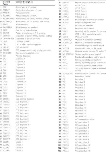
The data set contains about 8 million records of hos-pital stays, with 126 clinical and nonclinical data ele-ments for each visit (table 1). Nonclinical eleele-ments include patient demographics, hospital identification, admission date, zip code, calendar year, total charges and length of stay. Clinical elements include procedures, procedure categories, diagnosis codes and diagnosis categories. Every record contains a vector of 15 diagno-sis codes. The diagnodiagno-sis codes are represented using the

(3)

Table 1 HCUP data elements

Element Name

Element Description

1 AGE Age in years at admission

2 AGEDAY Age in days (when age > 1 year)

3 AMONTH Admission month

4 ASOURCE Admission source (uniform)

5 ASOURCEUB92 Admission source (UB-92 standard coding)

6 ASOURCE_X Admission source (as received from source)

7 ATYPE Admission type

8 AWEEKEND Admission day is a weekend

9 DIED Died during hospitalization

10 DISCWT Weight to discharges in AHA universe

11 DISPUB92 Disposition of patient (UB-92 standard coding)

12 DISPUNIFORM Disposition of patient (uniform)

13 DQTR Discharge quarter

14 DRG DRG in effect on discharge date

15 DRG18 DRG, version 18

16 DRGVER DRG grouper version used on discharge date

17 DSHOSPID Data source hospital identifier

18 DX1 Principal diagnosis

19 DX2 Diagnosis 2

20 DX3 Diagnosis 3

21 DX4 Diagnosis 4

22 DX5 Diagnosis 5

23 DX6 Diagnosis 6

24 DX7 Diagnosis 7

25 DX8 Diagnosis 8

26 DX9 Diagnosis 9

27 DX10 Diagnosis 10

*33 DXCCS1 CCS: principal diagnosis

*34 DXCCS2 CCS: diagnosis 2

48 ECODE1 E code 1

49 ECODE2 E code 2

50 ECODE3 E code 3

51 ECODE4 E code 4

Table 1 HCUP data elements(Continued)

52 ELECTIVE Elective versus non-elective admission

53 E_CCS1 CCS: E Code 1

57 FEMALE Indicator of sex

58 HOSPID HCUP hospital identification number

59 HOSPST Hospital state postal code

60 KEY HCUP record identifier

61 LOS Length of stay (cleaned)

62 LOS_X Length of stay (as received from source)

63 MDC MDC in effect on discharge date

64 MDC18 MDC, version 18

65 MDNUM1_R Physician 1 number (re-identified)

66 MDNUM2_R Physician 2 number (re-identified)

67 NDX Number of diagnoses on this record

68 NECODE Number of E codes on this record

69 NEOMAT Neonatal and/or maternal DX and/or PR

70 NIS_STRATUM Stratum used to sample hospital

71 NPR Number of procedures on this record

72 PAY1 Primary expected payer (uniform)

73 PAY1_X Primary expected payer (as received from source)

74 PAY2 Secondary expected payer (uniform)

75 PAY2_X Secondary expected payer (as received from source)

76 PL_UR_CAT4 Patient Location: Urban-Rural 4 Categories

77 PR1 Principal procedure

78 PR2 Procedure 2

79 PR3 Procedure 3

80 PR4 Procedure 4

81 PR5 Procedure 5

82 PR6 Procedure 6

83 PR7 Procedure 7

84 PR8 Procedure 8

85 PR9 Procedure 9

86 PR10 Procedure 10

92 PRCCS1 CCS: principal procedure

93 PRCCS2 CCS: procedure 2

(4)

symptom, or cause of death. There are numerous codes, over 14,000 ICD-9 codes and 3,900 procedures codes.

In addition, every record contains a vector of 15 diag-nosis category codes. The diagdiag-nosis categories are com-puted using the Clinical Classification Software (CCS) developed by HCUP in order to categorize the ICD-9 diagnosis and procedure codes. CCS collapsed these codes into a smaller number of clinically meaningful categories, called diagnosis categories. Every ICD-9 code has a corresponding diagnosis category and every

category contains a set of ICD-9 codes. We denote each of the 259 disease categories by a value between 1 and 259. In Figure 1 we show an example of disease category ("Breast cancer”) and some of the ICD-9 codes included in it (174.0 -"Malignant neoplasm of female breast”, 174.1-Malignant neoplasm of central portion of female breast”, 174.2-Malignant neoplasm of upper-inner quad-rant of female breast”, 233.0-"Carcinoma in situ of breast and genitourinary system”).

Demographics such as age, race and sex are also included in the data set. Figure 2 shows the distribution of patients across age, race and sex.

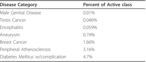
The data set is highly imbalanced. The imbalance rate ranges across diseases from 0.01-29.1%. 222 diagnosis categories occurs in less than 5% of the patients and only 13 categories occur in more than 10% of the patients. In table 2 we show the top 10 most prevalent disease categories and in table 3 we show some of the rarest diseases present in the 2005 HCUP data set.

One limitation of the 2005 HCUP data set is the arbi-trary order in which the ICD-9 codes and disease cate-gories were listed. The codes were not listed in the chronological order according to the date they were diagnosed. Also, the data set does not provide anon-ymous patient identifier, which could be used to check if multiple records belong to the same patient or to determine the elapsed time between diagnoses.

Data Pre-processing

The data set was provided in a large ASCII file contain-ing the 7,995,048 records. The first step was to parse the data set, randomly selectNrecords and extract a set of relevant features. Every record is a sequence of char-acters that are not delimited. However, the data set instructions specifies the starting column and the ending column in the ASCII file for each data element (length of data element). HCUP provides a SAS program to parse the data set, but we chose to develop our own program to perform the parsing.

Table 1 HCUP data elements(Continued)

107 PRDAY1 Number of days from admission to PR1

122 RACE Race (uniform)

123 TOTCHG Total charges (cleaned)

124 TOTCHG_X Total charges (as received from source)

125 YEAR Calendar year

126 ZIPInc_Qrtl Median household income quartile for patient’s ZIP Code

Complete list of 126 HCUP data elements. The elements marked with“*” (rows 33-47) are the ones used in the classification as input variables. *HCUP data elements used in the classification

(5)

Feature Selection

For every record, we extracted the age, race, sex and 15 diagnosis categories. Every record is represented as ad

= 262 dimensional feature vector. Features 1-259 are binary, one for each disease category. The remaining three features are age, race and sex. We denote the sam-ples that contain a given disease category as“active”and the remaining ones as“inactive”. The active and inactive data samples are defined only from the point of view of the disease being classified. A snippet of the data set is presented in table 4. For example, in table 4, sample 1 is active for disease category 50, while sample N is inactive.

While, in general, using only disease categories may not lead to a valid disease prediction, the approach pre-sented in this paper needs to be seen in the larger con-text of our TigerPlace eldercare research [11]. By integrating large public data sets (such as the one used in this paper) with monitoring sensors and electronic health records (EHR) data, we can achieve the required prediction precision for an efficient delivery of tailored medical information.

Learning from Imbalanced Data

A data set is class-imbalanced if one class contains sig-nificantly more samples than the other. For many dis-ease categories, the unbalance rate ranges between 0.01-29.1% (that is, the percent of the data samples that belong to the active class). For example, (see table 3) only 3.16% of the patients have Peripheral Atherosclero-sis. In such cases, it is challenging to create an appropri-ate testing and training data sets, given that most classifiers are built with the assumption that the test data is drawn from the same distribution as the training data [12].

Presenting imbalanced data to a classifier will produce undesirable results such as a much lower performance on the testing that on the training data. Among the clas-sifier learning techniques that deal with imbalanced data we mention oversampling, undersampling, boosting, bagging and repeated random sub-sampling [13,14]. In

the next section we describe the repeated random sub-sampling method that we employ in this paper.

Repeated Random Sub-Sampling

Repeated random sub-sampling was found to be very effective in dealing with data sets that are highly imbal-anced. Because most classification algorithms make the assumption that the class distribution in the data set is uniform, it is essential to pay attention to the class dis-tribution when addressing medical data. This method divides the data set into active and inactive instances, from which the training and testing data sets are gener-ated. The training data is partitioned into sub-samples with each sub-sample containing an equal number of instances from each class, except for last sub-sample (in some cases). The classification model is fitted repeatedly on every sub-sample and the final result is a majority voting over all the sub-samples.

In this paper we used the following repeated random sub-sampling approach. For every target disease we ran-domly choose Nsamples from the original HCUP data set. TheN samples are divided into two separate data sets,N1 active data samples and N0 inactive data

sam-ples, whereN1+ N0 =N. The testing data will contain

30% active samplesN1 (TsN1) while the remaining 70%

will be sampled from theN0 (TsN0) inactive samples.

The 30/70 ratio was chosen by trial-and-error. The training data set will contain the remaining active sam-ples (TrN1) and inactive samples (TrN0).

Since the training data is highly imbalanced (TrN1

>>TrN0), the TrN0 samples are partitioned into NoS

training sub-samples, where NoS is the ratio between

TrN0 andTrN1. Every training sub-sample has equal

number of instances of each class. The training active samples (TrN1) are fixed among all the training data

sub-samples, while the inactive samples will be sampled without replacement fromTrN0. There will beNoS

(6)

voting” approach to determine the final class member-ships (see Algorithm 1 in Additional File 1: Appendix). A diagram describing the process of RF and the sub-sampling procedure is presented in Figure 3.

Random Forest

RF is an ensemble learner, a method that generates many classifiers and aggregates their results. RF will cre-ate multiple classification and regression (CART) trees, each trained on a bootstrap sample of the original train-ing data and searches across a randomly selected subset of input variables to determine the split. CARTs are bin-ary decision trees that are constructed by splitting the data in a node into child nodes repeatedly, starting with the root node that contains the whole learning sample [15]. Each tree in RF will cast a vote for some inputx, then the output of the classifier is determined by major-ity voting of the trees (algorithm 2 in Additional File 1: Appendix). RF can handle high dimensional data and use a large number of trees in the ensemble. Some important features of RF are [16]:

1. It has an effective method for estimating missing data.

2. It has a method, weighted random forest (WRF), for balancing error in imbalanced data.

3. It estimates the importance of variables used in the classification.

Chen et al. [17], compared WRF and balanced random

forest (BRF) on six different and highly imbalanced data sets. In WRF, they tuned the weights for every data set, while in BRF, they changed the votes cutoff for the final prediction. They concluded that BRF is computationally more efficient than WRF for imbalanced data. They also found that WRF is more vulnerable to noise compared to BRF. In this paper, we used RF without tuning the class weights or the cutoff parameter.

Splitting Criterion

Like CART, RF uses the Gini measure of impurity to select the split with the lowest impurity at every node [18]. Gini impurity is a measure of the class label distri-bution in the node. The Gini impurity takes values in [0, 1], where 0 is obtained when all elements in a node are of the same class. Formally, the Gini impurity mea-sure for the variable X= {x1,x2, ...,xj} at nodet, wherej

is the number of children at nodet, Nis the number of samples, nci is the number of samples with value xi

belonging to class c, aiis the number of samples with

value xi at node t, then the Gini impurity is given by

[15]

Itxi

= 1−

c

c=0

nci

ai 2

(1)

The Gini index of a split is the weighted average of the Gini measure over the different values of variableX, which is given by

Gini(t,X)=

j

i=1

ai

NI

txi

(2)

The decision of the splitting criterion will be based on the lowest Gini impurity value computed among them

variables. In RF, each tree employs a different set of m

variables to construct the splitting rules.

Variable Importance

One of the most important features of RF is the output of the variable importance. Variable importance mea-sures the degree of association between a given variable and the classification result. RF has four measures for the variable importance: raw importance score for class 0, raw importance score for class 1, decrease in accuracy and the Gini index. To estimate variable importance for some variable j, the out-of-bag (OOB) samples are passed down the tree and the prediction accuracy is recorded. Then the values for variablejare permuted in the OOB samples and the accuracy is measured again. These calculations are carried out tree by tree as the RF is constructed. The average decrease in accuracy of these permutations is then averaged over all the trees and is used to measure the importance of the variable j.

Table 2 The 10 most prevalent diseases categories

Disease Category Prevalence

Hypertension 29.1%

Coronary Atherosclerosis 27.65%

Hyperlipidemia 14.46%

Dysrhythmia 14.35%

Other Circulatory Diseases 12.02%

Diabetes mellitus no complication 12%

Anemia 11.93%

The top 10 most prevalent diseases among the 8 million samples; it shows the percentage of the samples having that disease.

Table 3 Some of the most imbalanced diseases categories

Disease Category Percent of Active class

Male Genital Disease 0.01%

Testis Cancer 0.046%

Encephalitis 0.059%

Aneurysm 0.74%

Breast Cancer 1.66%

(7)

If the prediction accuracy decreases substantially, then that suggests that the variablej has strong association with the response [19]. After measuring the importance of all the variables, RF will return a ranked list of the variable importance.

Formally, let btbe the OOB samples for tree t, tÎ

{1,..., ntree}, y’ti is the predicted class for instance i

before the permutation in tree t and y’ti,a is the pre-dicted class for instance i after the permutation. The variable importanceVI for variablejin treetis given by

VIt_j=

N i=1βtI

yi=y

_t

t

|βt| −

N i=1βtI

yi=y

_t

i,α

|βt| (3)

The raw importance value for variable jis then aver-aged over all trees in the RF.

VIj= ntree

t=1 VItm

ntree (4)

The variable importance used in this paper is the Mean Decrease Gini (MDG), which is based on the Gini splitting criterion discussed earlier. The MDG measure the

decreaseΔI(equation 1) that results from the splitting. For two class problem, the change inI(equation 6) at nodetis defined as the class impurity (equation 5) minus the weight average of Gini measure (equation 2) [20,21].

I(t)= 1−

c

c=0 _n

i

N

2

(5)

I(t)=I(t)−Gini(t,X) (6)

The decrease in Gini impurity is recorded for all the nodestin all the trees (ntree) in RF for all the variables and Gini Importance (GI) is then computed as [20].

GI=

ntree

t

I(t) ₍₇₎

Classification with Repeated Random Sub-Sampling Training the classifier on a data set that is small and highly imbalanced will result in unpredictable results as

Table 4 Sample Dataset, the bolded column (Cat. 50) represents the category to predict

Cat. 1

Cat. 2

Cat. 3

.... Cat. 50

.... Cat. 257 Cat. 258 Cat. 259 Age Race Sex

Patient 1 0 0 0 .... 1 .... 0 1 1 69 3 0

. .

PatientN 1 0 0 .... 0 .... 1 0 0 55 1 1

(8)

discussed in earlier sections. To overcome this issue, we used repeated random sub-sampling. Initially, we con-struct the testing data and the NoS training data sub-samples. For each disease, we train NoS classifiers and test all of them on the same data set. The final labels of the testing data are computed using a majority voting scheme.

Model Evaluation

To evaluate the performance of the RF we compared it to SVM on imbalanced data sets for eight different chronic diseases categories. Two sets of experiments were carried out:

Set I: We compared RF, boosting, bagging and SVM performance with repeated random sub-sampling. Both classifiers were fitted to the same training and testing data and the process was repeated 100 times. The ROC curve and the average AUC for each clas-sifier were calculated and compared. To statistically compare the two ROC curves we employed an Ana-lysis of Variance (ANOVA) approach [22] where the standard deviation of each AUC was computed as:

SE=

θ (1−θ)+Cp−1 Q1−θ2

+(Cn−1)

Q2−θ2

CpCn

, (8)

where Cp, Cn, θ are the number positive instances,

negative instances and the AUC, respectively and

Q1= θ

(2−θ),Q2= 2∗θ2

(1 +θ). (9)

Set II: In this experiment we compare RF, bagging, boosting and SVM performance without the sam-pling approach. Without samsam-pling the data set is highly imbalanced, while sampling should improve the accuracy since the training data sub-samples fitted to the model are balanced. The process was again repeated 100 times and the ROC curve and the average AUC were calculated and compared.

Results

We performed the classification using R, which is open source statistical software. We used R Random Forest (randomForest), bagging (ipred), boosting (caTools) and SVM (e1071) packages. There are two parameters to choose when running a RF algorithm: the number of trees (ntree) and the number of randomly selected vari-ables (mtry). The number of trees did not significantly influence the classification results. This can be seen in Figure 4, where we ran RF for different ntreevalues to

predict breast cancer. As we see from Figure 4, the sen-sitivity of the classification did not significantly change once ntree>20. The number of variables randomly sampled as candidates at each split (mtry) was chosen as the square root of the number of features (262 in our case), hence mtrywas set to 16. Palmer et al. [23] and Liaw et al. [24] also reported that RF is usually insensi-tive to the training parameters.

For SVM we used a linear kernel, termination criter-ion (tolerance) was set to 0.001,epsilonfor the insensi-tive-loss function was 0.1 and the regularization term (cost) was set to 1. Also, we left bagging and boosting with the default parameters.

We randomly selectedN = 10,000 data points from the original HCUP data set. We predicted the disease risks on 8 out of the 259 disease categories. Those cate-gories are: breast cancer, type 1 diabetes, type 2 dia-betes, hypertension, coronary atherosclerosis, peripheral atherosclerosis, other circulatory diseases and osteoporosis.

Result set I: Comparison of RF, bagging, boosting and SVM

RF, SVM, bagging and boosting classification were per-formed 100 times and the average area under the curve (AUC) was measured (ROC curves for the four classi-fiers for diabetes with complication, hypertension and breast cancer are shown in Figure 5, Figure 6 and Figure 7, respectively). The repeated random sub-sampling approach has improved the detection rate considerably. On seven out of eight disease categories RF outper-formed the other classifiers in terms of AUC (table 5). In addition to ROC comparison, we used ANOVA [22] as mentioned earlier to statistically compare the ROC of boosting and RF, since both of these classifiers scored the highest in terms of AUC. ANOVA results compar-ing RF ROC and boostcompar-ing ROC are summarized in table 6. The lower thepvalue is the more significant the dif-ference between the ROCs is. The results of ANOVA test tells us that although RF outperformed boosting in terms of AUC, that performance was only significant in three diseases only (high prevalence diseases). The pos-sible reason for performance difference insignificance for the other 5 diseases (mostly low prevalence diseases) might be the low number of active samples available in our sampled dataset. For example, for breast cancer we would have about 166 cases available.

(9)

detailed physical, physiological, and laboratory examina-tions for each patient. The AUC for their classification scheme I and II was 83.47% and 73.81% respectively. We also predicted diabetes with complications and with-out complications and the AUC values were 94.31% and 87.91% respectively (Diabetes without complication ROC curve in Figure 5).

Davis et al. [8] used clustering and collaborative filtering to predict disease risks of patients based on their medical history. Their algorithm generates a ranked list of diseases

in the subsequent visits of that patient. They used an HCUP data set, similar to the data set we used. Their sys-tem predicts more than 41% of all the future diseases in the top 20 ranks. One reason for their low system perfor-mance might be that they tried to predict the exact ICD-9 code for each patient, while we predict the disease category. Zhang et al. [10] performed classification on breast cancer metastasis. In their study, they used two pub-lished gene expression profiles. They compared multiple methods (logistic regression, SVM, AdaBoost, Figure 4RF behaviour when the number of trees (ntree) varies. This plot shows how sensitivity in RF varies as the number of trees (ntree) varies, we variedntreefrom 1-1001 in intervals of 25 and measured the sensitivity at every interval. Sensitivity ranged from 0.8457 whenntree= 1 and 0.8984 whenntree= 726. In our experiments we usedntree= 500 since thentreedid not have a large affect on accuracy forntree>1.

Figure 5ROC curve for diabetes mellitus. ROC curve for diabetes mellitus comparing SVM, RF, boosting and bagging.

(10)

LogitBoost and RF). In the first data set, the AUC for SVM and RF was 88.6% and 89.9% respectively and for the second data set 87.4% and 93.2%. The results we obtained for breast cancer prediction for RF were 91.23% (ROC curve in Figure 7).

Mantzaris et al [9] predicted osteoporosis using multi-layer perceptron (MLP) and probabilistic neural network (PNN). Age, sex, height and weight were the input vari-ables to the classifier. They reported a prognosis rate on the testing data of 84.9%. One the same disease, we reported an AUC for RF of 87%.

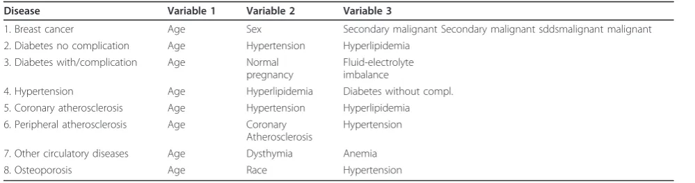
One of the important features of the RF approach is the computation of the importance of each variable (feature). We used Mean Decrease Gini (Equations 5, 6, 7) measure to achieve the variable importance (table 7). Variables with high importance have strong associa-tion with the predicassocia-tion results. For example, Man-tzaris et al. [9] mentioned that osteoporosis (row 8) is more prevalent in people older than 50 and occurs in women more than men and that agrees with the first and forth important variables (age and sex) reported by RF (Table 7). Another example is diabetes with complication (row 3) that often presents with fluid-electrolyte imbalance and it’s incidence is inversely correlated with a normal pregnancy.

Result set II: Sampling vs. non-sampling

In this section we show that classification with sampling outperforms standalone classifiers on the HCUP data set (table 8). RF, bagging, boosting and SVM with sampling have higher ROC curves and reaches a detection rate of 100% faster than the standalone classifiers. For

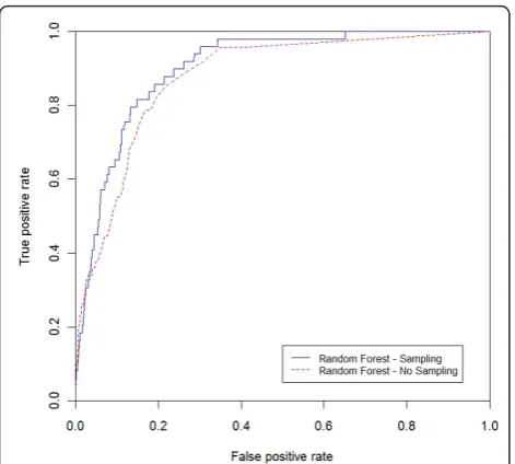
demonstration purposes, we included the comparisons for RF with and without sampling for three disease cate-gories, breast cancer, other circulatory diseases and per-ipheral atherosclerosis (ROC curve in Figure 8, Figure 9, and Figure 10). Table 8 describes the results for the non-sampling classification for the four mentioned classifiers.

Discussion

Disease prediction is becoming an increasingly impor-tant research area due to the large medical datasets that are slowly becoming available. While full featured clini-cal records are hard to access due to privacy issues, dei-dentified large public dataset are still a valuable resource for at least two reasons. First, they may provide popula-tion level clinical knowledge. Second, they allow the data mining researcher to develop methodologies for clinical decision support systems that can then be employed for electronic medical records. In this study, we presented a disease prediction methodology that employs random forests (RF) and a nation-wide deiden-tified public dataset (HCUP). We show that, since no national medical warehouse is available to date, using nation-wide datasets provide a powerful prediction tool. In addition, we believe that the presented methodology can be employed with electronic medical records, if available.

Figure 7 ROC curve for breast cancer. ROC curve for breast cancer comparing both SVM, RF, boosting and bagging.

Table 5 RF, SVM, bagging and boosting performance in terms of AUC on eight disease categories

Disease RF SVM Bagging Boosting

Breast cancer 0.9123 0.9063 0.905 0.8886

Diabetes no complication 0.8791 0.8417 0.8568 0.8607 Diabetes with/complication 0.94317 0.9239 0.9294 0.9327

Hypertension 0.9003 0.8592 0.8719 0.8842

Coronary Atherosclerosis 0.9199 0.8973 0.887 0.9026 Peripheral Atherosclerosis 0.9095 0.8972 0.8967 0.9003 Other Circulatory Diseases 0.7899 0.7591 0.7669 0.7683

Osteoporosis 0.87 0.867 0.8659 0.8635

Table 6 Statistical comparison of RF and boosting ROC curves, the lower the value the more significant the difference is

Disease pvalue

Breast cancer 0.8057

Diabetes no complication 0.3293

Diabetes with/complication 0.6266

Hypertension 0.2

Coronary Atherosclerosis 0.2764

Peripheral Atherosclerosis 0.8203

Other Circulatory Diseases 0.566

(11)

To test our approach we selected eight chronic dis-eases with high prevalence in elderly. We performed two sets of experiments (set I and set II). In set I, we compared RF to other classifiers with sampling, while in set II we compared RF to other classifiers without sub-sampling. Our results show that we can predict diseases with an acceptable accuracy using the HCUP data. In addition, the use of repeated random sub-sampling is useful when dealing with highly imbalanced data. We also found that incorporating demographic information increased the area under the curve by 0.33-10.1%.

Some of the limitations of our approach come from limitations of the HCUP data set such as the arbitrary order of the ICD-9 codes and lack of patient identifica-tion. For example, since the ICD-9 codes are not listed in chronological order according to the date they were diagnosed, we inherently use future diseases in our pre-diction. This explains, in part, the high accuracy of our prediction. In addition, the HCUP data set does not pro-vide anonymous patient identifier, which can be used to check if multiple records belong to the same patient and to estimate the time interval between two diagnoses. Hence we might use the data for the same patient mul-tiple times.

Additionally, the data set does not include the family history; rather it includes the individual diagnosis history which is represented by the diseases categories.

Conclusions

In this study we used the NIS dataset (HCUP) created by AHRQ. Few researchers have utilized the NIS dataset for disease predictions. The only work we found on dis-ease prediction using NIS data was presented by Davis et al. [5], in which clustering and collaborative filtering was used to predict individual disease risks based on medical history. In this work we provided extensive proof that RF can be successfully used for disease pre-diction in conjunction with the HCUP dataset.

Table 7 Top four most importance variable for the eight disease categories

Disease Variable 1 Variable 2 Variable 3

1. Breast cancer Age Sex Secondary malignant Secondary malignant sddsmalignant malignant

2. Diabetes no complication Age Hypertension Hyperlipidemia

3. Diabetes with/complication Age Normal

pregnancy

Fluid-electrolyte imbalance

4. Hypertension Age Hyperlipidemia Diabetes without compl.

5. Coronary atherosclerosis Age Hypertension Hyperlipidemia

6. Peripheral atherosclerosis Age Coronary

Atherosclerosis

Hypertension

7. Other circulatory diseases Age Dysthymia Anemia

8. Osteoporosis Age Race Hypertension

Table 8 RF, SVM, bagging and boostingperformance without sub-sampling in terms of AUC on eight disease categories

Disease RF SVMSVM Bagging Boosting

Breast cancer 0.8793 0.5 0.5085 0.836

Diabetes no complication 0.8567 0.5 0.4749 0.8175 Diabetes with/complication 0.9084 0.648 0.4985 0.8278

Hypertension 0.8893 0.6908 0.4886 0.8515

Coronary Atherosclerosis 0.9193 0.6601 0.4945 0.8608 Peripheral Atherosclerosis 0.8872 0.5 0.4925 0.8279 Other Circulatory Diseases 0.7389 0.5 0.4829 0.6851

Osteoporosis 0.7968 0.5 0.4931 0.8561

(12)

The accuracy achieved in disease prediction is com-parable or better than the previously published results. The average RF AUC obtained across all disease was about 89.05% which may be acceptable in many applica-tions. Additionally, unlike many other published results were they focus on predicting one specific disease, our method can be used to predict the risk for any disease. Finally, we consider the results obtained with the

proposed method adequate for our intended use, which is tailored health communication.

Additional material

Additional file 1: Appendix. This file contains two algorithms. Algorithm 1, which describes the repeated random sub-sampling and algorithm 2 which briefly explains the general random forest for classification.

Acknowledgements

The authors would like to thank the University of Missouri Bioinformatics Consortium for providing us with a Supercomputer account to run the experiments.

Author details

1

Department of Computer Science, University of Missouri, Columbia, Missouri, USA.2_{Department of Statistics, University of Missouri, Columbia,} Missouri, USA.3Department of Health Management and Informatics, University of Missouri, Columbia, Missouri, USA.

Authors’contributions

MK is the main author of this paper. He designed and wrote the code, ran the experiments, collected the results and analyzed them, and drafted the manuscript. Professor SC developed and contributed to the design of the experiments, specially the repeated random sub-sampling approach and reviewed the manuscript. MP, MK_’s advisor, provided the data, helped in designing the experiments, provided continuous feedback on the paper, mainly the result section and reviewed the manuscript.

All authors have read and approved the final manuscript.

Competing interests

The authors declare that they have no competing interests.

Received: 28 September 2010 Accepted: 29 July 2011 Published: 29 July 2011

References

1. Yu W,et al:Application of support vector machine modeling for prediction of common diseases: the case of diabetes and pre-diabetes. BMC Medical Informatics and Decision Making2010,10(1):16.

2. Hebert P,et al:Identifying persons with diabetes using Medicare claims data.American Journal of Medical Quality1999,14(6):270.

3. Fuster V,et al:Medical Underwriting for Life InsuranceMcGraw-Hill_’s AccessMedicine; 2008.

4. Yi T, Guo-Ji Z:The application of machine learning algorithm in underwriting process.Machine Learning and Cybernetics, 2005. Proceedings of 2005 International Conference on2005.

5. Cohen E,et al:Cancer coverage in general-audience and black newspapers.Health Communication2008,23(5):427-435.

6. HCUP Project:Overview of the Nationwide Inpatient Sample (NIS)2009 [http://www.hcup-us.ahrq.gov/nisoverview.jsp].

7. Moturu ST, Johnson WG, Huan L:Predicting Future High-Cost Patients: A Real-World Risk Modeling Application.Bioinformatics and Biomedicine, 2007. BIBM 2007. IEEE International Conference on2007.

8. Davis DA, Chawla NV, Blumm N, Christakis N, Barabási AL:Proceeding of the 17th ACM conference on Information and knowledge management. Predicting individual disease risk based on medical history2008, 769-778. 9. Mantzaris DH, Anastassopoulos GC, Lymberopoulos DK:Medical disease

prediction using Artificial Neural Networks.BioInformatics and BioEngineering, 2008. BIBE 2008. 8th IEEE International Conference on2008. 10. Zhang W,et al:A Comparative Study of Ensemble Learning Approaches

in the Classification of Breast Cancer Metastasis.Bioinformatics, Systems Biology and Intelligent Computing, 2009. IJCBS_‘09. International Joint Conference on2009, 242-245.

11. Skubic M, Alexander G, Popescu M, Rantz M, Keller J:A Smart Home Application to Eldercare: Current Status and Lessons Learned, Technology and Health Care.2009,17(3):183-201.

Figure 10ROC curve for peripheral atherosclerosis (sampling vs. non-sampling). ROC curve for peripheral atherosclerosis comparing RF with the sampling and non-sampling approach.

(13)

12. Provost F:Machine learning from imbalanced data sets 101.Proceedings of the AAAI_’2000 Workshop on Imbalanced Data Sets2000.

13. Japkowicz N, Stephen S:The class imbalance problem: A systematic study.Intelligent Data Analysis2002,6(5):429-449.

14. Quinlan JR:Bagging, boosting, and C4. 5.Proceedings of the National Conference on Artificial Intelligence1996, 725-730.

15. Breiman L,et al: InClassification and regression trees. Volume 358. Wadsworth. Inc., Belmont, CA; 1984.

16. Breiman L:Random forests.Machine learning2001,45(1):5-32. 17. Chen C, Liaw A, Breiman L:Using random forest to learn imbalanced data

University of California, Berkeley; 2004.

18. Breiman L, others:Manual-Setting Up, Using, and Understanding Random Forests V4. 0.2003 [ftp://ftpstat.berkeley.edu/pub/users/breiman]. 19. Hastie T,et al:The elements of statistical learning: data mining, inference and

prediction2009, 605-622.

20. Bjoern M,et al:A comparison of random forest and its Gini importance with standard chemometric methods for the feature selection and classification of spectral data.BMC Bioinformatics10.

21. Mingers J:An empirical comparison of selection measures for decision-tree induction.Machine learning1989,3(4):319-342.

22. Bradley AP:The use of the area under the ROC curve in the evaluation of machine learning algorithms.Pattern Recognition1997,30:1145-1159. 23. Palmer D,et al:Random forest models to predict aqueous solubility.J

Chem Inf Model2007,47(1):150-158.

24. Liaw A, Wiener M:Classification and Regression by randomForest.

Pre-publication history

The pre-publication history for this paper can be accessed here: http://www.biomedcentral.com/1472-6947/11/51/prepub

doi:10.1186/1472-6947-11-51

Cite this article as:Khaliliaet al.:Predicting disease risks from highly imbalanced data using random forest.BMC Medical Informatics and Decision Making201111:51.

Submit your next manuscript to BioMed Central and take full advantage of:

• Convenient online submission

• Thorough peer review

• No space constraints or color figure charges

• Immediate publication on acceptance

• Inclusion in PubMed, CAS, Scopus and Google Scholar

• Research which is freely available for redistribution