RESEARCH ARTICLE
10.1002/2014WR016062
Model selection on solid ground: Rigorous comparison of nine
ways to evaluate Bayesian model evidence
Anneli Sch€oniger1, Thomas W€ohling2,3, Luis Samaniego4, and Wolfgang Nowak5
1Center for Applied Geoscience, University of T€ubingen, T€ubingen, Germany,2Water and Earth System Science (WESS)
Competence Cluster, University of T€ubingen, T€ubingen, Germany,3Lincoln Environmental Research, Lincoln Agritech, Hamilton, New Zealand,4Department Computational Hydrosystems, Helmholtz-Zentrum for Environmental Research—
UFZ, Leipzig, Germany,5Institute for Modelling Hydraulic and Environmental Systems (LS3)/SimTech, University of Stuttgart, Stuttgart, Germany
Abstract
Bayesian model selection or averaging objectively ranks a number of plausible, competing con-ceptual models based on Bayes’ theorem. It implicitly performs an optimal trade-off between performance in fitting available data and minimum model complexity. The procedure requires determining Bayesian model evidence (BME), which is the likelihood of the observed data integrated over each model’s parameter space. The computation of this integral is highly challenging because it is as high-dimensional as the num-ber of model parameters. Three classes of techniques to compute BME are available, each with its own chal-lenges and limitations: (1) Exact and fast analytical solutions are limited by strong assumptions. (2)Numerical evaluation quickly becomes unfeasible for expensive models. (3) Approximations known as infor-mation criteria (ICs) such as the AIC, BIC, or KIC (Akaike, Bayesian, or Kashyap inforinfor-mation criterion, respec-tively) yield contradicting results with regard to model ranking. Our study features a theory-based intercomparison of these techniques. We further assess their accuracy in a simplistic synthetic example where for some scenarios an exact analytical solution exists. In more challenging scenarios, we use a brute-force Monte Carlo integration method as reference. We continue this analysis with a real-world application of hydrological model selection. This is a first-time benchmarking of the various methods for BME evalua-tion against true soluevalua-tions. Results show that BME values from ICs are often heavily biased and that the choice of approximation method substantially influences the accuracy of model ranking. For reliable model selection, bias-free numerical methods should be preferred over ICs whenever computationally feasible.
1. Introduction
The idea of model validation is to objectively scrutinize a model’s ability to reproduce an observed data set and then to falsify the hypothesis that this model is a good representation for the system under study [Popper, 1959]. If this hypothesis cannot be rejected, the model may be considered for predictive purposes. Modelers have been encouraged for centuries to create multiple such working hypotheses instead of limiting them-selves to the subjective choice of a single conceptual representation, therewith avoiding the ‘‘dangers of parental affection for a favorite theory’’ [Chamberlin, 1890]. These dangers include a significant underestima-tion of predictive uncertainty due to the neglected conceptual uncertainty (uncertainty in the choice of a most adequate representation of a system). Recognizing conceptual uncertainty as a main contribution to overall predictive uncertainty [e.g.,Burnham and Anderson, 2003;Gupta et al., 2012;Clark et al., 2011;Refsgaard et al., 2006] makes model selection an ‘‘integral part of inference’’ [Buckland et al., 1997]. The quantification of conceptual uncertainty is of importance in a variety of scientific disciplines, e.g., in climate change modeling [Murphy et al., 2004;Najafi et al., 2011], weather forecasting [Raftery et al., 2005], hydrogeology [Rojas et al., 2008;Poeter and Anderson, 2005;Ye et al., 2010a], geostatistics [Neuman, 2003;Ye et al., 2004], vadose zone hydrology [W€ohling and Vrugt, 2008], and surface hydrology [Ajami et al., 2007;Vrugt and Robinson, 2007;
Renard et al., 2010], to name only a few selected examples from the field of water resources.
Different strategies have been proposed to develop alternative conceptual models, assess their strengths and weaknesses, and to test their predictive ability. Bayesian model averaging (BMA) [Hoeting et al., 1999] is a formal statistical approach which allows comparing alternative conceptual models, testing their adequacy, combining their predictions into a more robust output estimate, and quantifying the contribution of
Key Points:
The choice of BME evaluation method influences the outcome of model ranking
Out of the ICs, the KIC@MAP is the most consistent one
For reliable model selection, there is still no alternative to numerical methods
Correspondence to:
A. Sch€oniger,
Citation:
Schoniger, A., T. W€ €ohling, L. Samaniego, and W. Nowak (2014), Model selection on solid ground: Rigorous comparison of nine ways to evaluate Bayesian model evidence,Water Resour. Res.,50, 9484–9513, doi:10.1002/2014WR016062.
Received 27 JUN 2014 Accepted 30 OCT 2014
Accepted article online 4 NOV 2014 Published online 19 DEC 2014
This is an open access article under the terms of the Creative Commons Attribution-NonCommercial-NoDerivs License, which permits use and distribution in any medium, provided the original work is properly cited, the use is non-commercial and no modifications or adaptations are made.
Water Resources Research
conceptual uncertainty to the overall prediction uncertainty. The BMA approach is based on Bayes’ theo-rem, which combines a prior belief about the adequacy of each model with its performance in reproducing a common data set. It yields model weights that represent posterior probabilities for each model to be the best one from the set of proposed alternative models. Based on the weights, it allows for a ranking and quantitative comparison of the competing models. Hence, BMA can be understood as a Bayesian hypothe-sis testing framework, merging the idea of classical hypothehypothe-sis testing with the ability to test several alterna-tive models against each other in a probabilistic way. The principle of parsimony or ‘‘Occam’s razor’’ [e.g.,
Angluin and Smith, 1983] is implicitly followed by Bayes’ theorem, such that the posterior model weights reflect a compromise between model complexity and goodness of fit (also known as the bias-variance trade-off [Geman et al., 1992]). BMA has been adopted in many different fields of research, e.g., sociology [Raftery, 1995], ecology [Link and Barker, 2006], hydrogeology [Li and Tsai, 2009], or contaminant hydrology [Troldborg et al., 2010], indicating the general need for such a systematic model selection procedure.
The drawback of BMA is, however, that it involves the evaluation of a quantity called Bayesian model evi-dence (BME). This integral over a model’s parameter space typically cannot be computed analytically, while numerical solutions come at the price of high computational costs. Various authors have suggested and applied different approximations to the analytical BMA equations to render the procedure feasible.Neuman
[2003] proposes a Maximum Likelihood Bayesian Model Averaging approach (MLBMA), which reduces com-putational effort by evaluating Kashyap’s information criterion (KIC) for the most likely parameter set instead of integrating over the whole parameter space. This is especially compelling for high-dimensional applications (i.e., models with many parameters). If prior knowledge about the parameters is not available or vague, a further simplification leads to the Bayesian information criterion or Schwarz’ information crite-rion (BIC) [Schwarz, 1978;Raftery, 1995]. The Akaike information criterion (AIC) [Akaike, 1973] originates from information theory and is frequently applied in the context of BMA in social research [Burnham and Ander-son, 2003] for its ease of implementation. Previous studies have revealed that these information criteria (IC) differ in the resulting posterior model weights or even in the ranking of the models [Poeter and Anderson, 2005;Ye et al., 2008, 2010a, 2010b;Tsai and Li, 2010, 2010;Singh et al., 2010;Morales-Casique et al., 2010;
Foglia et al., 2013]. This implies that they do not reflect the true Bayesian trade-off between performance and complexity, but might produce an arbitrary trade-off which is not supported by Bayesian theory and cannot provide a reliable basis for Bayesian model selection.Burnham and Anderson[2004] conclude that
‘‘. . .many reported studies are not appropriate as a basis for inference about which criterion should be
used for model selection with real data.’’ The work ofLu et al. [2011] has been a first step into clarifying the so far contradictory results by comparing the KIC and the BIC against a Markov chain Monte Carlo (MCMC) reference solution for a synthetic geostatistical application.
Our study aims to advance this endeavor by rigorously assessing and comparing a more comprehensive set of nine different methods to evaluate BME. In specific, we will highlight their theoretical derivation, compu-tational effort, and approximation accuracy. As representatives of mathematical approximations, we con-sider the AIC, AICc (bias-corrected AIC), and BIC in our comparison. We further include the KIC evaluated at the maximum likelihood parameter estimate (KIC@MLE) as introduced in MLBMA, and an alternative formu-lation that is evaluated at the maximum a posteriori parameter estimate instead (KIC@MAP). We also con-sider three types of Monte Carlo integration techniques (simple Monte Carlo integration, MC; MC integration with importance sampling, MC IS; MC integration with posterior sampling, MC PS) and a very recent approach called nested sampling (NS) as representatives of numerical methods. By pointing out and comparing the important features and assumptions of these mostly well-known techniques, we are able to argue which methods are truly suitable for BME evaluation, and which ones are suspected to yield inaccu-rate results. We then present a simplistic synthetic, linear test case where an exact analytical expression for BME exists. With this first-time benchmarking of the different BME evaluation methods against the true solution, we close a significant gap in the model selection literature.
compute BME exists. We therefore generate a reference solution by brute-force MC integration, after having proven its suitability as reference solution in the linear case. In a third step, we present a real-world applica-tion of hydrological model selecapplica-tion. We chose this applicaapplica-tion such that the model selecapplica-tion task is still rel-atively simple and unambiguous. Even in this case the deficiencies of some of the evaluation methods become apparent. Our systematic investigation of methods to determine BME takes an important next step toward robust model selection in agreement with Bayes’ theorem,heaving it up on solid ground.
We summarize the statistical framework of BMA in section 2 and discuss assets and drawbacks of the avail-able techniques to determine BME in section 3. In section 4, we present the first-time benchmarking of the featured methods on the simplistic test case. Section 5 compares the approximation performance in a real-world hydrological model selection problem. We summarize our findings and formulate recommendations on which methods to use for reliable model selection in even more complex situations in section 6.
2. Bayesian Model Averaging Framework
We formulate the BMA equations according toHoeting et al. [1999]. All probabilities and statistics are implic-itly conditional on the set of considered models. While the suite of models is a subjective choice that lies in the responsibility of the modeler, it is the starting point for a systematic procedure to account for model uncertainty based on objective likelihood measures.
Let us considerNmplausible, competing modelsMk. The posterior predictive distribution of a quantity of interestugiven the vector of observed datayocan be expressed as:
pðujyoÞ5X
Nm
k51
pðujyo;MkÞP Mð kjyoÞ (1)
withpðjyoÞrepresenting a conditional probability distribution andP Mð kjyoÞbeing discrete posterior model weights. The weights can be interpreted as the Bayesian probability of the individual models to be the best representation of the system from the set of considered models.
The model weights are given by Bayes’ theorem:
P Mð kjyoÞ5
pðyojMkÞP Mð kÞ
XNm
i51pðyojMiÞP Mð iÞ
; (2)
with the prior probability (or rather subjective model credibility)P Mð kÞthat modelMkcould be the best one (the most plausible, adequate, and consistent one) in the set of modelsbeforeany observed data have been consid-ered. A ‘‘reasonable, neutral choice’’ [Hoeting et al., 1999] could be equally likely priorsP Mð kÞ51=Nmif there is lit-tle prior knowledge about the assets of the different models under consideration. The denominator in equation (2) is the normalizing constant of the posterior distribution of the models. It is easily obtained by determination of the individual weights. It could even be neglected, since all model weights are normalized by the same con-stant, so that the ranking of the individual models against each other is fully defined by the proportionality:
P Mð kjyoÞ /pðyojMkÞP Mð kÞ: (3)
pðyojMkÞrepresents the BME term as introduced in section 1 and is also referred to asmarginal likelihoodor
prior predictivebecause it quantifies the likelihood of the observed data based on the prior distribution of the parameters:
pðyojMkÞ5
ð
Uk
pðyojMk;ukÞpðukjMkÞduk; (4)
pðukjMk;yoÞ5
pðyojMk;ukÞpðukjMkÞ
pðyojMkÞ
: (5)
pðyojMkÞacts as a model-specific normalizing constant for the posterior of the parameterspðukjMk;yoÞ. As a matter of fact, evaluatingpðyojMkÞfor any given model is a major nuisance in Bayesian updating, and MCMC methods have been developed with the goal to entirely avoid its evaluation. However, in order to evaluate BME, this normalizing constant has to be determined, which is the challenge addressed in the cur-rent study. Rearranging equation (5) yields the alternative formulation for equation (4):
pðyojMkÞ5
pðyojMk;ukÞpðukjMkÞ
pðukjMk;yoÞ
: (6)
MacKay[1992] refers to the twofold evaluation of Bayes’ theorem (equations (2) and (4) or (6)) as the ‘‘two levels of inference’’ in Bayesian model averaging: the first level is concerned with finding the posterior distri-bution of the models, the second level with finding the posterior distridistri-bution of each model’s parameters (or rather its normalizing constant).
The integration over the full parameter space in equation (4) can be an exhaustive calculation, especially for high-dimensional parameter spacesUk. The alternative of computing the posterior distribution of the param-eters (defining the ‘‘calibrated’’ parameter space, equation (5)) is similarly demanding in high-dimensional applications. Analytical solutions are available only under strongly limiting assumptions. In general, mathe-matical approximations or numerical methods have to be drawn upon instead. We discuss and compare the nine different methods to compute BME in the following section and assess their accuracy in section 4.
3. Available Techniques to Determine BME
We will adopt the notation ofKass and Raftery[1995] for equation (4):
Ik5pðyojMkÞ5
ð
Uk
pðyojMk;ukÞpðukjMkÞduk (7)
and denote any approximation to the true BME valueIkasIk. After explaining two formulations of the ana-lytical solution in detail in section 3.1, we examine mathematical approximations in the form of ICs in sec-tion 3.2. Finally, we discuss assets and drawbacks of selected numerical evaluasec-tion methods in secsec-tion 3.3 and summarize our preliminary findings from this theoretical comparison in section 3.4. All BME evaluation methods featured in this study are listed with their underlying assumptions in Table 4. All approximation methods (i.e., the nine nonanalytical approaches) follow equation (7) to evaluate BME. We do not use equa-tion (6) here, since typically for medium to highly parameterized applicaequa-tions, the multivariate probability density of posterior parameter realizations cannot be estimated. Knowing the posterior parameter distribu-tion up to its normalizing constant (as in MCMC methods, see secdistribu-tion 3.3.3) does not suffice here since the normalizing constant is actually the targeted quantity itself.
3.1. Analytical Solution
The Bayesian integral or BMEIkfor modelMkcan be evaluated analytically for exponential family distribu-tions with conjugate priors [see e.g.,DeGroot, 1970]. Thus, analytical solutions for BME are available, if the observed datayoare measurements of the model parametersukor a linear function thereof and a conju-gate prior (i.e., the prior parameter distribution is in the same family as the posterior parameter distribution) exists. This is generally not the case in realistic applications. However, we will briefly outline the analytical solution to BME under these restrictive and simple conditions, before we discuss other evaluation methods that are not limited by these strong assumptions in sections 3.2 and 3.3.
We will focus here on the special case of a linear modelMkwith a linear model operatorHkrelating multi-Gaussian parametersukto multivariate Gaussian distributed variablesyk:
Mk:yk5Hkuk: (8)
The prior parameter distribution is defined as a normal distributionpð Þ Nuk ðuk;CuuÞwith the prior mean
The residuals5yo2yksignify any type of error associated with the data set and the models, e.g., measure-ment errors and model errors. Here we assume the models to be perfect (free of model errors) and only measurement errors to be relevant, and adopt a Gaussian model Nð0;RÞwith a diagonal matrixR rep-resenting the covariance matrix for uncorrelated measurement errors. This results in a Gaussian likelihood functionpðyojMk;ukÞ Nðyk;RÞ. Using the theory of linear uncertainty propagation [e.g.,Schweppe, 1973] and the stated assumptions, BME can be directly evaluated for any given data setyofrom the Gaussian distribution:
Ik5pðyojMkÞ NHkuk;Cyy1R; (9)
withCyy5HkCuuHTk.
As an alternative way to determine BME analytically, the posterior distribution of the parameters can be derived since the Gaussian distribution family is self-conjugate [Box and Tiao, 1973]. In general, the likeli-hoodLof the observed data given the prior parameter space of modelMkcan be written as a function of the parametersLðMk;ukjyoÞ[Fisher, 1922]. Note that the likelihood function is not necessarily a proper probability density function with respect touk, because it does not necessarily integrate to one. With the assumptions of Gaussian measurement noise and a linear model, the likelihood can be expressed as a Gauss-ian function of the parametersLðMk;ukjyoÞ Nðu^k;Cu^^uÞwithu^k5 HTkHk
21
HTkyoandC^uu^5 HTkR21Hk
21
. The mean of the distribution,u^k, is the maximum likelihood estimate (MLE) and (in this case) also the estimate obtained by ordinary least squares regression. It represents the parameter vector that yields the best possible fit to the observed data to be achieved by modelMk.
The combination of a Gaussian prior distribution and a Gaussian likelihood function yields an analytical expression for the posterior distributionpðukjyo;MkÞ Nðu~k;Cu~~uÞ, which is again Gaussian withu~k5C~u~u
C2^u^u1u^k1C2uu1uk
andC~u~u5 C2^uu^11C2uu1
21
. Under the current set of assumptions, the mean of the posterior distribution,u~k, is the maximum a posteriori estimate (MAP). The MAP represents those parameter values that are the most likely ones for modelMk, taking into account both prior belief about the distribution of the parameters and the performance in fitting the observed data. For a derivation of these statistics, see e.g.,Box and Tiao[1973].
With the posterior parameter distribution, the quotient in equation (6) (Bayes’ theorem rewritten to solve for the normalizing constant, equivalent to the integral in equation (7)) can be determined for any given valueuk;iwithin the limits ofpð Þuk .
3.2. Mathematical Approximation
If no analytical solution exists to the application at hand, equation (7) can be approximated mathematically, e.g., by a Taylor series expansion followed by a Laplace approximation. We briefly outline this approach in section 3.2.1 and then discuss the derivation of the KIC (section 3.2.2) which is based on this approximation. In this context, it becomes more evident how Occam’s razor works in BMA (section 3.2.3). The BIC (section 3.2.4) represents a truncated version of the KIC. Another mathematical approximation, which is based on information theory, results in the AIC(c) (section 3.2.5). We contrast the expected impact of the different IC formulations on model selection in section 3.2.6.
3.2.1. Laplace Approximation
The idea of the Laplace method [De Bruijn, 1961] is to approximate the integral by defining a simpler mathe-matical function for a subinterval of the original parameter space, assuming that the contribution of this neighborhood almost makes up the whole integral. Here a Gaussian posterior distribution is assumed as sim-plification to the unknown distribution. This is a suitable approximation if the posterior distribution is highly peaked around its mode (or maximum)u~. This assumption holds, if a large data set with a high information content is available for calibration. Expanding the logarithm of the integrand in equation (7) by a Taylor series about the posterior modeu~k(i.e., the MAP), neglecting third-order and higher-order terms, taking the exponent again and finally performing the integration with the help of the Laplace approximation yields:
I
k5LðMk;u~kjyoÞpðu~kjMkÞð2pÞNp;k=2jR~j1=2; (10)
with the likelihood functionLðMk;u~kjyoÞ, the prior densitypðu~kjMkÞ, and the number of parametersNp;k.
TheNp;kxNp;kmatrixR52~ @
2hð Þu
@u2
h i21
ju5u~is the negative inverse Hessian matrix of second derivatives and
actually Gaussian posterior (see section 3.1). For details on the Laplace approximation in the field of Bayes-ian statistics and an analysis of its asymptotic errors, please refer toTierney and Kadane[1986].
If the parameter prior is little informative, the expansion could also be carried out about the MLEu^kinstead of the MAP~uk. This approximation will be less accurate in general, with the deterioration depending on the distance between the MAP and MLE estimators. However, the MLE may be easier to find than the MAP with standard optimization routines. The corresponding approximation takes the following form:
I
k5LðMk;u^kjyoÞpðu^kjMkÞð2pÞNp;k=2jR^j1=2: (11)
The inverse of the covariance matrixR^is the observed Fisher information matrix evaluated at the MLE,
F52@2l
@u2ju5u^, withlbeing the log-likelihood function [Kass and Raftery, 1995].
If the normalized (per observation) Fisher information is used,F15F=Ns;R^equals½F1Ns215N1sF211[Ye et al., 2008]:
I
k5LðMk;u^kjyoÞpðu^kjMkÞð2pÞNp;k=2jF^j21=2
5LðMk;u^kjyoÞpð^ukjMkÞ 2p
Ns
Np;k=2
j^F1j21=2 :
(12)
For clarity in notation, model indices are omitted here for the covariance matrices and for the Fisher infor-mation matrix.
The presented mathematical approximations to the Bayesian Integral (equation (7)) are typically known in the shape of ICs, i.e., as22lnI
k. We subsequently discuss the three most commonly used ICs in the BMA framework. They all generally aim at identifying the optimal bias-variance trade-off in model selection, but differ in their theoretical derivation and therefore in their accuracy with respect to the theoretically optimal trade-off according to Bayes’ theorem.
3.2.2. Kashyap Information Criterion
The Kashyap information criterion (KIC) directly results from the approximation defined in equation (12) by applying22lnI
k[Kashyap, 1982]:
KIC^u522lnLðMk;u^kjyoÞ22lnpðu^kjMkÞ1Np;kln
Ns
2p1lnjF^1j: (13)
The KIC is applied within the framework of MLBMA [Neuman, 2002]. By means of this approximation, MLBMA is a computationally feasible alternative to full Bayesian model averaging if knowledge about the prior of parameters is vague. For applications of MLBMA, seeNeuman[2003],Ye et al. [2004],Neuman et al. [2012], and references therein.
If an estimate of the postcalibration covariance matrixC^u^uis obtainable, equation (11) can be drawn upon instead:
KIC^u522lnLðMk;u^kjyoÞ22lnpðu^kjMkÞ2Np;kln 2ð pÞ2lnjC^u^uj: (14)
Ye et al. [2004] point toward the close relationship of theKIC^uwith the original Laplace approximation, but prefer the evaluation at the MLE, because it is in line with traditional MLE-based hydrological model selec-tion and parameter estimaselec-tion routines.Neuman et al. [2012] appreciate that MLBMA ‘‘admits but does not require prior information about the parameters’’ and include prior information in their likelihood optimiza-tion routine, which makes it de facto a MAP estimaoptimiza-tion routine. We strongly advertise the latter variant, because the Laplace approximation originally involves an expansion about the MAP instead of the MLE, and we understand prior information on the parameters as a vital part of Bayesian inference. Therefore, we pro-pose to explicitly evaluate the KIC at the MAP:
KIC~u5 22lnLðMk;~ukjyoÞ
|fflfflfflfflfflfflfflfflfflfflfflfflfflffl{zfflfflfflfflfflfflfflfflfflfflfflfflfflffl}
NLL
22lnpð~ukjMkÞ
|fflfflfflfflfflfflfflfflfflfflffl{zfflfflfflfflfflfflfflfflfflfflffl} 1
2Np;kln 2ð pÞ
|fflfflfflfflfflfflfflfflffl{zfflfflfflfflfflfflfflfflffl} 2
2lnjC~u~uj |fflfflfflfflffl{zfflfflfflfflffl}
3 |fflfflfflfflfflfflfflfflfflfflfflfflfflfflfflfflfflfflfflfflfflfflfflfflfflfflfflfflfflfflfflfflffl{zfflfflfflfflfflfflfflfflfflfflfflfflfflfflfflfflfflfflfflfflfflfflfflfflfflfflfflfflfflfflfflfflffl}
Occam factor
: (15)
evaluation at the MAP is consistent with the Laplace approach to approximate the Bayesian integral and, in case of an actually Gaussian parameter posterior, will yield accurate results; this does not hold if the approx-imation is evaluated at the MLE. If the assumption of a Gaussian posterior is violated, it needs to be assessed how the different evaluation points affect the already inaccurate approximation. We will investigate the dif-ferences in performance between the KIC@MLE and our proposed KIC@MAP in section 4.
3.2.3. Interpretation Via Occam’s Razor
In equation (15), we have distinguished different terms of the Laplace approximation in the formulation of the KIC@MAP. They can be interpreted within the context of BMA, and if the assumption of a Gaussian pos-terior parameter distribution is satisfied, this represents an interpretation of the ingredients of BME (or more specifically, minus twice the logarithm of BME). It incorporates a measure of goodness of fit (the nega-tive log-likelihood term, NLL) and three penalty terms that account for model dimensionality (dimension of the model’s parameter space). These three terms are referred to as Occam factor [MacKay, 1992].
The Occam factor reflects the principle of parsimony or Occam’s razor: If any number of competing models shows the same quality of fit, the least complex one should be used to explain the observed effects. Any additional parameter is considered to be fitted to noise in the observed data and might lead to low parame-ter sensitivities and poor predictive performance (due to little robustness of the estimated parameparame-ters). Syn-thesizing the discussions byNeuman[2002, 2003],Ye et al. [2004], andLu et al. [2011], and explicitly transferring them to the expansion about the MAP, we make an attempt to explain the role of the three terms that are contained in the Occam factor.
The parameter priorpðu~kjMkÞ(term 1) implicitly penalizes a growing complexity in that it gives a lower probability density to models with larger parameter spaces (largerNp;k), since high-dimensional densities have to dilute their total probability mass of unity within a larger space. Thus, a more complex model with its smaller prior parameter probabilities will obtain a higher value of the criterion or a decreased value of BME, which will compromise its chances to rule out its competitors according to Occam’s razor.
The opposite is true for2Np;kln 2ð pÞ(term 2): here, an increase in dimensionality yields a decrease of the KIC or an increase in model evidence. This term is actually part of the normalizing factor of a Gaussian prior distribution and thus partially compensates the effect of (1).
Finally,jC~u~uj(term 3) accounts for the curvature of the posterior distribution. A strong negative curvature, i.e., a very narrow posterior distribution, represents a high information content in the data with respect to the calibration of the parameters. A narrow posterior leads to a low value for the determinant and thus to a decrease in model evidence or an increase of the KIC. This might seem counter-intuitive at first, but has to be interpreted from the viewpoint that if the data provide a high information content, the resulting likeli-hood function shall be narrow, and thus, its peak value shall also be high. The determinant is thus a partially compensating counterpart to the NLL term. If two competing models achieve the same likelihood, but differ in their sensitivity to the data, the one with a smaller sensitivity will be chosen because of its robustness [Ye et al., 2010b].
3.2.4. Bayesian Information Criterion
The Bayesian information criterion (BIC) or Schwarz information criterion [Schwarz, 1978] is a simplification to equation (13) in that it only retains terms that vary withNs:
BIC522lnLðMk;u^kjyoÞ1Np;klnNs: (16)
Applying the KIC or BIC for modelselection(as opposed to averaging) is consistent as the assigned weight for the true model (if it is a member of the considered set of models) converges to unity for an infinite data set size. The truncated form (BIC) still seems to perform reasonably well for model identification or explana-tory purposes [Koehler and Murphree, 1988]. It is also much less expensive to evaluate than the KIC for mod-els with high-dimensional parameter spaces, since the evaluation of the covariance matrix is not required.
3.2.5. Akaike Information Criterion
The Akaike information criterion (AIC) or, as originally entitled, ‘‘an information criterion,’’ originates from information theory (as opposed to the Bayesian origin of the KIC and BIC), but has frequently been applied in the framework of BMA [e.g.,Poeter and Anderson, 2005]. It is derived from the Kullback-Leibler (KL) diver-gence that measures the loss of information when using an alternative modelMkwith a predictive density functiong Yð jMk;ukÞinstead of the ‘‘true’’ model with predictive density functionf Yð Þ, withYbeing a ran-dom variable from the true densityfof the same sizeNsas the observed data setyo:
DKLðf;gÞ5
ð
f Yð Þln f Yð Þ
g Yð jMk;ukÞ
dY
5Ef½lnf Yð Þ2Ef½lng Yð jMk;ukÞ:
(17)
The first term in the second line of equation (17) is an unknown constant that drops out when comparing differences in the expected KL-information for the competing models in the set [e.g.,Kuha, 2004].Akaike
[1973, 1974] argued that the second term, called relative expected KL-information, can be estimated using the MLE. For reasons not provided here, this estimator is biased byNp;k, the number of parameters in the modelMk. Correcting this bias and multiplying by22 yields the AIC [Burnham and Anderson, 2004]. The AIC formulation contains the NLL term as an expression for the goodness of fit and a penalty term for the num-ber of parameters:
AIC522lnLðMk;u^kjyoÞ12Np;k: (18)
Compared to the BIC in equation (16), the penalty term for the number of parametersNp;kis less severe. For data set sizesNs>7, BIC favors models with less parameters than AIC, since its penalty termNp;klnNs becomes larger than the AIC’s 2Np;k.
For a finite data set sizeNs, a second-order bias correction has been suggested [Sugiura, 1978;Hurvich and
Tsai, 1989]:
AICc5AIC12Np;k Np;k11
Ns2Np;k21
: (19)
Among others,Burnham and Anderson[2004] suggest using the corrected formulation for data set sizes
Ns<40Np;k. For increasing data set sizes, the AICc converges to the AIC.
The posterior Akaike model weight is derived from:
P Mð kjyoÞ5
expð20:5䉭kÞ
XNm
i51expð20:5䉭iÞ
5XexpN ð20:5AICkÞ m
i51expð20:5AICiÞ
; (20)
with䉭k5AICk2AICminor䉭k5AICck2AICcmin, respectively. Based on its theoretical derivation, the absolute value ofAICkorAICckhas no explanatory power [Burnham and Anderson, 2004], only the difference䉭kwith respect to the lowestAICkorAICckcan be interpreted. The BIC or KIC, in contrast, are a direct approximation to BME (equation (7)) and therefore yield meaningful values, also in interpretation as absolute values.
The AIC seems to perform well for predictive purposes, with a tendency to over-fit observed data [see e.g.,
Koehler and Murphree, 1988;Claeskens and Hjort, 2008]. This tendency is supposedly less severe for the bias-corrected AICc. Both versions of the AIC do not converge to the true model for an infinite data set size. The reason is that, with an increasing amount of data, the model chosen by AIC(c) will increase in complexity, potentially beyond the complexity of the true model (if it exists) [Burnham and Anderson, 2004].
et al. [2010], andLu et al. [2011]. In the following, we will summarize the main theoretical differences in the BME approximation by these ICs.
3.2.6. Theoretical Comparison of IC Approximations to BME
Based on equation (10), the Laplace approximated BME can be divided into the likelihood and the Occam factorOF(see section 3.2.3):
I
k5LðMk;~ukjyoÞpðu~kjMkÞð2pÞNp;k=2jR~j1=25LðMk;u~kjyoÞOF: (21)
The ICs analyzed here all share the same approximation for the goodness of fit term based on the MLE. The only exception is the KIC@MAP, which is evaluated at the MAP instead of at the MLE. However, they all differ in their approximation to the OF. The OF represents the penalty for the dimensionality of a model or what we call thesharpness of Occam’s razor. For the different ICs, it is given by:
OFKIC;~u5pðu~jMkÞð2pÞNp;k=2jC~u~uj1=2
OFKIC;^u5pðu^jMkÞð2pÞNp;k =2j
C^u^uj1 =2
OFBIC5Ns2Np;k=2
OFAIC5exp2Np;k
OFAICc5exp 2Np;k2 1 2
2Np;k Np;k11
Ns2Np;k21
:
(22)
The OF as approximated by KIC does not explicitly account for data set size, yetNstypically influences the curvature of the posterior probability (or the likelihood function) and thus implicitly affectsjC~u~uj1=2(or jC^u^uj1
=2). In contrast, AICc and BIC explicitly take data set sizeN
sin account, but do not evaluate the sensitiv-ity of the calibrated parameter set via the curvature. The effects of these differences on the accuracy of the BME approximation will be demonstrated exemplarily on two test case applications in sections 4 and 5.
3.3. Numerical Evaluation
Numerical evaluation offers a second alternative to determine BME, if no analytical solution is available or if one mistrusts the approximate character of the ICs. A comprehensive review of numerical methods to eval-uate the Bayesian integral (equation (7)) is given byEvans and Swartz[1995]. In the following, we will shortly review selected state-of-the-art methods and discuss their strengths and limitations. Note that conventional efficient integration schemes (e.g., adaptive Gaussian quadrature) are limited to low-dimensional applica-tions [Kass and Raftery, 1995]. In this study, we focus on numerical methods that can also be applied to highly complex models (models with large parameter spaces) in order to provide a useful discussion for a broad range of research fields and applications.
3.3.1. Monte Carlo Integration
Simple Monte Carlo integration [Hammersley, 1960] evaluates the integrand at randomly chosen pointsuk;i in parameter space. These parameter setsuk;iare randomly drawn from their prior distributionpðukjMkÞ. The integral (or expected value over parameter space, cf. equation (4)) is then determined as the mean value of the evaluated likelihoods (sometimes referred to asarithmetic mean approach):
I
k5
1
N
XN
i51
L Mk;uk;ijyo
; (23)
with the number of Monte Carlo (MC) realizationsN. For large ensemble sizesNand a friendly overlap of the parameter prior and the likelihood function, this method will provide very accurate results. For high-dimensional parameter spaces, however, a sufficient (converging) ensemble might come at a high or even prohibitive computational cost. If the likelihood function is sharp compared to the prior distribution, only very few integration points will contribute a high likelihood value to the integral (makingLa very skewed variable), and the numerical uncertainty in the approximated integral might be large.
3.3.2. Monte Carlo Integration With Importance Sampling
distribution. Thus, the mass of the integral will be detected more likely by the sampling points. When draw-ing from a different distributionqthan the prior distributionp, the integrand in equation (7) must be expanded byq/q. This modifies equation (23) to:
I
k5
XN
i51wiL Mk;uk;ijyo
XN
i51wi
; (24)
with weightswi5p uk;ijMk
=q uk;ijMk
. The improvement achieved by importance sampling compared to simple MC integration will greatly depend on the choice of the importance functionq.
3.3.3. Monte Carlo Integration With Posterior Sampling
Developing this idea further, it could be most advantageous to draw parameter realizations from the poste-rior distributionpðukjyo;MkÞin order to capture the full mass of the integral. Sampling from the posterior distribution is possible, e.g., with the MCMC method [Hastings, 1970].
For posterior sampling, the approximation to the integral reduces to the harmonic mean of likelihoods [Newton and Raftery, 1994], also referred to as theharmonic mean approach:
I
k5
1
N
XN
i51
L Mk;uk;ijyo
21
" #21
: (25)
Equation (25) can be subject to numerical instabilities, due to small likelihoods that may corrupt the evalua-tion of the harmonic mean.
According to Jensen’s inequality [Jensen, 1906], sampling exclusively from the posterior parameter distribu-tion yields a biased estimator that overestimates BME. Thus, the harmonic mean approach should be seen as a trade-off between accuracy and computational effort. In order to avoid the instabilities of the harmonic mean approach by solving equation (6) instead, it would be necessary to estimate the posterior parameter probability density from the generated ensemble through kernel density estimators [e.g.,H€ardle, 1991], which is only possible for low-dimensional parameter spaces. We therefore do not investigate this alterna-tive option further within this study.
3.3.4. Integration in Likelihood Space With Nested Sampling
The main challenge in evaluating BME lies in sufficiently sampling high-dimensional parameter spaces. A promising approach which avoids this challenge and instead samples the one-dimensional likelihood space is called nested sampling [Skilling, 2006]. The integral to obtain BME is written as:
Ik5pðyojMkÞ5
ð
LðMk;ukjyoÞdZ; (26)
whereZrepresents prior masspðukjMkÞdu. It is solved by discretizing intomlikelihood threshold values with the sequenceL1<L2<. . .<Lmand summing up over the corresponding prior mass pieces 1>Z1
>Z2>. . .>Zm>0 according to a numerical integration rule. How to find subsequent likelihood
thresh-olds is described inSkilling[2006].
One of the remaining challenges for this very recent approach lies in finding conforming samples above the current likelihood threshold. We followElsheikh et al. [2013] in utilizing a short random walk Markov chain starting from a random sample that overcame the previous threshold. However, instead of using the ratio of likelihoods as acceptance distribution, we take the ratio of prior probabilities instead, to ensure that new samples still conform with their prior. Another challenge lies in ending the procedure with a suitable termination criterion (e.g., stop if the increase in BME per iteration has flat-tened out or if the likelihood threshold cannot be overcome within a maximum number of MCMC steps).
3.4. Conclusions From Theoretical Comparison
From our comparison of the underlying assumptions for the nine BME evaluation methods considered here, we conclude that out of the ICs, the KIC@MAP is the most consistent one with BMA theory. It represents the true solution if the assumptions of the Laplace approximation hold (i.e., if the posterior parameter distribu-tion is Gaussian). The other ICs considered here represent simplificadistribu-tions of this approach or, in the case of the AIC(c), are derived from a different theoretical perspective and are therefore expected to show an infe-rior approximation quality. Among the numerical methods considered here, simple MC integration is the most generally applicable approach because it is bias-free and spares any assumptions on the shape of the parameter distribution, but is also the computationally most expensive one. The other numerical methods vary in their efficiency, but are expected to yield similarly accurate results, except for MC integration with posterior sampling, which yields a biased estimate. We will test these expectations on a synthetic setup in the following section. The underlying assumptions of the nine BME evaluation methods analyzed in this study are summarized in Table 4.
4. Benchmarking on a Synthetic Test Case
The nine methods to solve the Bayesian integral (equation (7)) differ in their accuracy and computational effort, as described in the previous section. To illustrate the differences in accuracy under completely con-trolled conditions, we apply the methods presented in section 3 to an oversimplified synthetic example. In a first step, we consider a setup with a linear model where an analytical solution exists. We create an ideal premise for the KIC@MAP and its variants (KIC@MLE and BIC) by using a Gaussian parameter posterior, which fulfills their core assumption. We designed this test case as a best-case scenario regarding the formance of these ICs: there is no less challenging case in which the information criteria could possibly per-form better. In a second step, we also consider nonlinear models of different complexity that violate this core assumption. Since in this case no analytical solution exists, we use brute-force MC integration as refer-ence for benchmarking. We designed this test case as an intermediate step toward real-world applications that typically entail nonlinear models and a higher number of parameters.
4.1. Setup and Implementation
In the first step, a linear modely5u1x1u2relates bivariate Gaussian distributed parametersu5½u1;u2 (slope and intersect of a linear function) to multi-Gaussian distributed predictionsyat measurement loca-tionsx. This linear model is tested against a synthetic data set. The synthetic truth underlying the data set is generated from the same model, but with slightly different parameter values than the prior mean. To obtain a synthetic data set, a random measurement error is added according to a Gaussian distribution
Nð0;RÞ.
For this artificial setup, BME can be determined analytically according to equations (9) (determining BME via linear uncertainty propagation) or 6 (solving Bayes’ theorem for BME). This exact value is used as reference for the approximate methods presented in section 3. In this simple case, the MAP,u~, and the MLE,u^, are known analytically. Also, the corresponding covariancesC~u~uandC^uu^are known. We allow the mathematical approximations to take advantage of this knowledge by evaluating them at these exact values. Normally, these quantities have to be approximated by optimization algorithms first. This initial step represents the computational effort needed to determine BME with mathematical approximations in the form of ICs, since the evaluation of their algebraic equations itself is very cheap. Here we are not concerned with the potential challenge to find these parameter estimates, but merely wish to remind the reader of this fact.
sampling are generated by the differential evolution adaptive metropolis adaptive MCMC scheme DREAM [Vrugt et al., 2008]. With DREAM, BME is approximated based on ensembles of 5000–1,000,000 parameter realizations. Convergence of the MCMC runs was monitored by the Gelman-Rubin criterion [Gelman and Rubin, 1992] and we chose to take the final 25% of the converged Markov chains as posterior ensemble. Nested sampling is per-formed with initial ensemble sizes of 10–10,000. A nested sampling run is complete if one of the two following termination criteria is reached. The first termination criterion stops the calculation if the current likelihood threshold could not be overcome within 100 MCMC steps with a scaling vectord50:05 ffiffiffiffiffiffiffiC11
p
; ffiffiffiffiffiffiffiC22 p
. The sec-ond termination criterion stops the calculation if the current BME estimate would not increase by more than 0.5% even if the current maximum likelihood value would be multiplied with the total remaining prior mass. This results in total ensemble sizes (summed over all iterations) of roughly 1000–1,000,000.
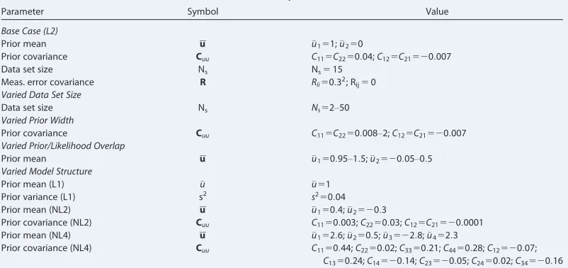
As a base case, we generate a synthetic data set of sizeNs515. Figure 1 shows the setup for the synthetic test case. The parameters used in the synthetic example are summarized in Table 1.
In our synthetic test case, the computational effort required for one model run is very low. This allows us to repeat the entire analysis for the base case and to average over 500 runs for each ensemble size in order to quantify the inherent numerical uncertainty in the results obtained from the numerical approximation methods. In the case of nested sampling, we additionally average over 200 random realizations of the prior mass shrinkage factor per run.
With the setup described above, we compare the performance of the different approximation methods in quantifying BME. Additionally, we study by scenario variations the impact of varied data set size and varied prior information (different mean values and variances of parameters) on the outcome of BME and on the performance of the different methods. The behavior of the mathematical approximations for small or large data set sizes has been touched upon in the literature [e.g.,Burnham and Anderson, 2004;Lu et al., 2011]. We will underpin these discussions by systematically increasing the data set size fromNs52 toNs550. Again, the same model is used to generate the synthetic truth as in the base case, and the measurements are taken at equidistant locations on the same interval ofx. To show the general behavior of the approxima-tion methods and to eliminate artifacts caused by a specific outcome of measurement error, we generate 200,000 perturbed data sets for each data set size and average over the results of these realizations.
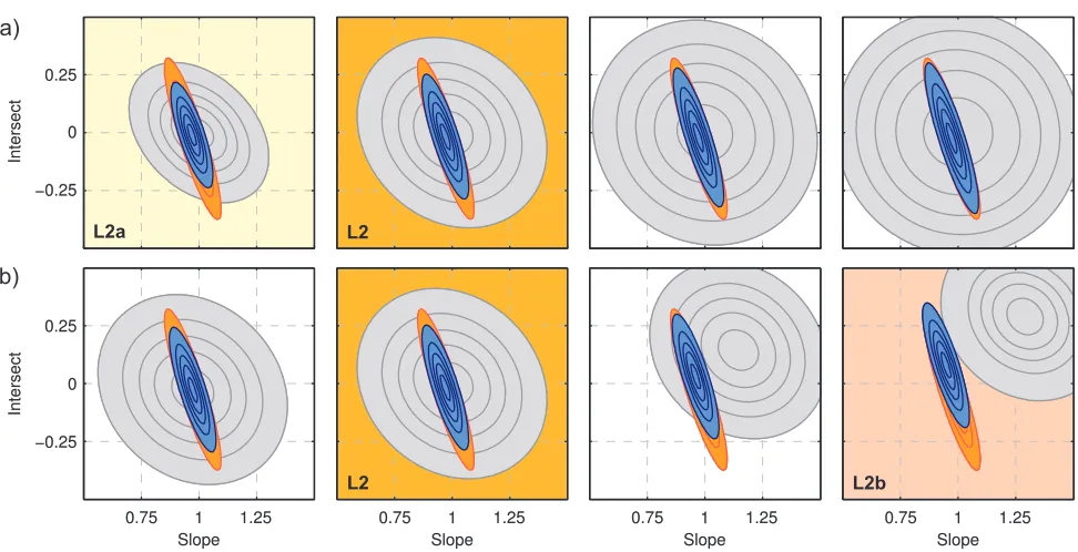
To our knowledge, the impact of prior information on the performance of BME approximation methods has not yet been studied in such a systematic approach. With the help of our synthetic test case, we can assess and then discuss this impact in a rigorous manner. Figure 2a visualizes the prior parameter densities, the likelihood func-tion, and the posterior densities for a range of prior widths, Figure 2b for different prior/likelihood overlaps. The second column represents the base case as described above. Variations in prior width are normalized as fractions of the base case variances (covariance is not varied), variations in overlap of prior and likelihood are measured as distance between the prior mean and the MLE. The varied parameter values are also listed in Table 1.
scattering) achieved by the other numerical methods is based on 500 repeated runs with ensemble sizes of 50,000, which might be con-sidered a reasonable compromise between accuracy and computational effort based on the findings from the first step of our synthetic test case. From the posterior parameter sam-ple generated by DREAM, we determine the MAP and the covariance matrix needed for the evaluation of the KIC@MAP. We obtain the respective ML statistics for the KIC@MLE from a DREAM run with uninformative prior distri-butions to cancel out the influence of the prior. We also evaluate the AIC(c) and the BIC at this parameter set.
For all cases (base case, varied data set size, varied prior information, varied model struc-ture), the error in BME approximation is quan-tified as a relative error
Erel5 jjI
i2Ijj
I ; (27)
with the subscriptirepresenting any of the discussed methods. In the case of numerical techniques, the averageErelvalue and its Bayesian confidence interval out of all repetitions is provided.
Finally, we determine the impact of BME approximation errors on model weights based on the same setup and implementation details as described for the investigation of the influence of model structure (section 4.5).
4.2. Results for the Base Case
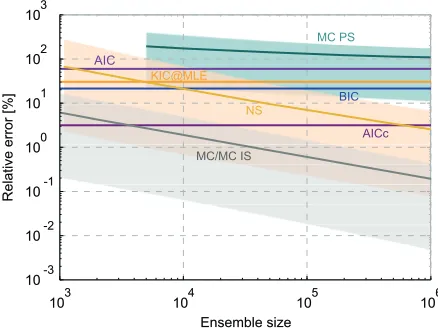
Figure 3 shows the relative error of BME approximations with respect to the analytical solution for the base case (see definition of parameters in section 4.1) as a function of ensemble size (number of model calls). Obviously, the accuracy of approximation improves for numerical methods when investing more computa-tional effort, i.e., when increasing the numerical ensemble size. The improvement includes both a reduction
0 1 2 3 4 5
0 2 4 6
Measurement location x
Prediction y
L1
Measurements
0 1 2 3 4 5
0 2 4 6
Measurement location x
Prediction y
L2 (base case) NL2
NL4
Figure 1.Synthetic test case setup. Measurements marked in black, prior estimate of linear (L1, L2) and nonlinear (NL2, NL4) models in solid lines, 95% Bayesian prediction confidence intervals in dashed lines of the respective color.
Table 1.Definition of Parameters Used in Different Scenarios of the Synthetic Test Casea
Parameter Symbol Value
Base Case (L2)
Prior mean u u151;u250
Prior covariance Cuu C115C2250:04;C125C21520:007
Data set size Ns Ns515
Meas. error covariance R Rii50:32; R
ij50
Varied Data Set Size
Data set size Ns Ns52–50
Varied Prior Width
Prior covariance Cuu C115C2250:008–2;C125C21520:007 Varied Prior/Likelihood Overlap
Prior mean u u150:95–1:5;u2520:05–0:5
Varied Model Structure
Prior mean (L1) u u51
Prior variance (L1) s2
s250:04
Prior mean (NL2) u u150:4;u2520:3
Prior covariance (NL2) Cuu C1150:003;C2250:03;C125C21520:0001
Prior mean (NL4) u u152:6;u250:5;u3522:8;u452:3
Prior covariance (NL4) Cuu C1150:44;C2250:02;C3350:21;C4450:28;C12520:07; C1350:24;C14520:14;C23520:05;C2450:02;C34520:16
a
in bias (error) and a reduction in variance (numerical uncertainty, shown as 95% Bayesian confidence inter-vals of the approximation error in Figure 3).
Simple MC integration (MC) and MC integration with importance sampling (MC IS) perform equally well for this setup. MC results improve linearly in quality in this log-log-plot, which complies with its well-known convergence rate ofOðN2s1=2Þ(Central Limit Theorem) [Feller, 1968]. MC integration with sampling from the posterior (MC PS), however, leads to a severe overestimation of BME as anticipated (see section 3.3.3) and does not improve linearly with ensemble size in log-log-space, but shows a slower convergence. It also pro-duces a much larger numerical uncertainty (keep in mind the logarithmic scale of the error axis). Note that the bias in BME approximation stems from the harmonic mean formulation and not from the sampling technique, because the posterior realizations generated with DREAM were checked to be consistent with the (in this case) known analytical posterior parameter distribution.
Nested sampling (NS) shows a similar approximation quality to MC integration, but is shifted on thexaxis, i.e., it is less efficient with regard to numerical ensemble sizes in this specific test case. The convergence behavior shown here might not be a general property of nested sampling, because we found that modifica-tions in the termination criteria significantly influence its approximation quality and uncertainty bounds. For this synthetic linear test case, we conclude that nested sampling is not as efficient as simple MC integration. It is also less reliable due to its somewhat arbitrary formulation with respect to the search for a replacement realization and the choice of termination criteria. In principle, it offers an alternative to simple MC integra-tion and might become more advantageous in high-dimensional parameter spaces. We will continue this discussion for the real-word hydrological test case (section 5) and draw some final conclusions in section 6.
other ICs yield approximation errors of 20– 60%. Figure 3 shows that, except for MC inte-gration with posterior sampling, the numeri-cal methods outperform all of the ICs evaluated at the MLE, if only enough realiza-tions are used.
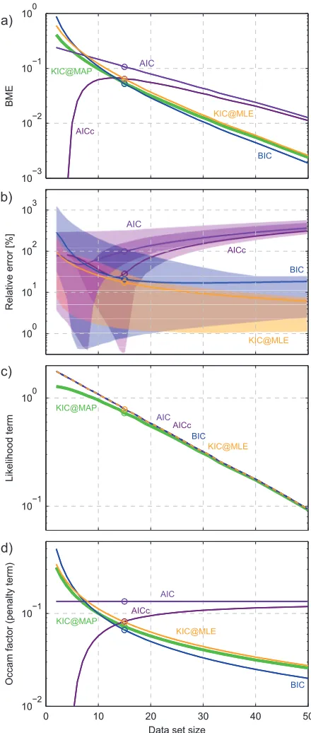
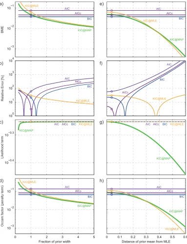
4.3. Results for Varied Data Set Size The approximation results as a function of data set size are shown in Figure 4. Since we have demonstrated that the numerical methods (except for posterior sampling) can approximate the true solution with arbitrary accuracy if only the invested computational power is large enough, we do not show their results here, as they would coincide with the solution of the KIC@MAP. Figure 4a shows the approximated BME values, while the rela-tive error in percent with respect to the ana-lytical solution is shown in Figure 4b.
The true BME curve (represented by the KIC@MAP here) is approximated quite well by both the KIC@MLE and by the BIC. However, while the KIC@MLE converges to the KIC@MAP with increasing data set size, the BIC does not. Its relative error with respect to the analytical solution becomes stable at more than 20%. This result is not in agreement with the findings ofLu et al. [2011], who confirmed the general belief that the BIC approaches the KIC with increasing data set size. In our case, the contribution of the terms dismissed by the BIC (see section 3.2) is still significant and hence produces a relevant deviation between the two BME approximations.
The AIC shows a linear dependence on data set size in this semilog plot. As expected, the AICc converges to the AIC with increasing data set size. Still, both variants of the AIC produce a relative error of more than 30%, which even increases with increasing data set size to more than 300% in this specific test case. Again, be reminded that the AIC(c) is only derived for comparing models with each other by the means of model weights, not as an approximation to the absolute BME value.
We investigate the reasons for the different behavior of the ICs over data set size by separating the likeli-hood term from the Occam factor penalty term (see section 3.2.6). Figure 4c shows how the true likelilikeli-hood term (here: KIC@MAP) is approximated by the other ICs. Obviously, approximating this term produces negli-gible errors if the data set size is reasonably large, i.e., if the MAP and the MLE almost coincide. The prob-lems in BME approximation clearly stem from the challenge of approximating the Occam factor (Figure 4d). The true Occam factor (or complexity penalty term) decreases with data set size. The KIC@MLE converges to this true behavior. The BIC is able to closely approximate the true curve, but does not yet converge to it in the range analyzed here. The penalty term of the AIC is a constant, which intersects the BIC’s penalty term curve atNs57 (see explanation in section 3.2.5). The penalty term of the AICc variant is converging to the constant AIC from below, i.e., it is increasing in contrast to the true, decreasing behavior. We conclude that the ICs differ substantially in the way they approximate the penalty term and therefore yield very different BME approxima-tions with huge relative errors observed for the AIC and AICc.
Note that the results forNs515 measurements, marked with circles in Figure 4, are similar, but not equal to the results we showed in Figure 3. This is due to the fact that to investigate the influence of data set size, we have marginalized over the random measurement error, while as a base case, we presented results for just one specific outcome of measurement error. We chose this scenario on purpose to illustrate that all those approximation methods which do not explicitly account for the sensitivity of the parameters to the specific data set, suffer from unpredictable behavior. The range of potential relative errors (95% Bayesian confidence intervals) over all 200,000 random realizations of measurement errors are shown as shaded areas in Figure 4b. It becomes clear that, up to a data set size of aboutNs520 in our test case, none of the specific ICs would be a reliable choice: the AIC, AICc, and BIC could potentially yield very low (<1%) or very
103 104 105 106
10 ¡ 3 10
¡ 2 10
¡ 1 100 101 102 103
Ensemble size
Relative error [%]
103 104 105 106
10 ¡-3 10
¡-2 10
¡-1 100 101 102 103
Ensemble size
Relative error [%]
BIC
AIC
AICc KIC@MLE
MC/MC IS
MC PS
NS
high (>100%) relative errors. Choosing the KIC@MLE is a more reliable choice, since it shows narrower bounds of potential relative errors, but still results in intolerable errors up to a data set size of about 30 in this case. We will elaborate on the question of how to make a safe choice of BME evaluation method in section 6.
4.4. Results for Varied Prior Information Next, we investigate the behavior of the ICs for varied prior information. Figure 5 compares the influence of the prior width (left column) with the influence of varied distance between the MLE and the prior mean, i.e., of a shifted prior (right column). Again, we present the BME approximation (Figures 5a and 5e) and its relative error (Figures 5b and 5f), and the KIC@MAP rep-resents the true solution. The AIC, AICc, and BIC approximations are constant over both variations, because they are not able to detect any information about the prior beyond the sheer number of parameters. In theory, however, increasing the prior width and moving the prior away from the area of high likelihood, both lead to a decrease in BME, which can be seen in the BME curve obtained by the KIC@MAP. While BME stabilizes at some point when increasing the prior width to a fully unin-formative prior, it falls steeply if the prior is shifted farther away. This is important to keep in mind, because also the systematic relative errors in approximation (Figures 5b and 5f) are much larger for the shifted prior.
Only the KIC@MLE is able to track the varia-tions in prior information and yields accept-able errors in both BME approximation and the approximation of the individual terms (likelihood term, Figures 5c and 5g, and penalty term, Figures 5d and 5h). Neverthe-less, this error is in the range of 10%. In the case of increased prior width, the KIC@MLE converges to the true solution because the MAP moves toward the MLE, and, at the same time, the posterior covariance is approximated more closely by the covari-ance around the MLE. In contrast, there is no such convergence behavior with decreasing distcovari-ance between the MLE and the prior mean, because in that case only the MAP moves toward the MLE, but the covariances do not coincide if the prior is still somewhat informative. Therefore, the solution of the KIC@MLE deviates from the true BME value even if the MAP is equal to the MLE, still producing a relative error of 30%.
10−3 10−2 10−1 100 BME 10−3 10−2 10−1 100 BME 100 101 102 103
Relative error [%]
100 101 102 103
Relative error [%]
10−1 100 Likelihood term 10−1 100 Likelihood term
0 10 20 30 40 50
10−2 10−1
Data set size
Occam factor (penalty term)
0 10 20 30 40 50
10−2 10−1
Data set size
Occam factor (penalty term)
KIC@MAP KIC@MLE AIC AICc BIC BIC AIC AICc KIC@MLE KIC@MLE AIC BIC AICc KIC@MAP KIC@MLE KIC@MAP AIC AICc BIC a) b) c) d)
For increasing distance between the MLE and the prior mean, the approximation of the likelihood term (Fig-ure 5g) by MLE-based criteria deteriorates significantly. Since neither the likelihood term nor the penalty term are adequately approximated by the AIC, AICc, or BIC, substantial errors in BME approximation arise. There are poles in the relative error curves, where they cut the analytical solution. These locations are, how-ever, dependent on the actual model at hand and on the outcome of the measurement error, and can therefore not be predicted a priori. Again, preferring any IC among AIC, AICc, and BIC as an approximation to BME is not a reliable choice as already pointed out when analyzing their performance over data set size. We will discuss implications of this finding in section 6.
10−3 10−2 10−1
10−3 10−2 10−1
BME
100 101 102 103 104
100 101 102 103 104
Relative Error [%]
10−0.4 10−0.3
10−0.4 10−0.3
Likelihood term
0 1 2 3 4 5
10−3 10−2 10−1
Fraction of prior width
0 1 2 3 4 5
10−3 10−2 10−1
Fraction of prior width
Occam factor (penalty term)
0 0.1 0.2 0.3 0.4 0.5 0.6
Distance of prior mean from MLE
0 0.1 0.2 0.3 0.4 0.5 0.6
Distance of prior mean from MLE KIC@MAP
KIC@MLE
AIC AICc
BIC
AIC
AICc
BIC
KIC@MAP
KIC@MLE
KIC@MLE KIC@MLE
AIC
AICc
BIC
AIC AICc
BIC
KIC@MLE
KIC@MAP
KIC@MAP
AIC AICc BIC
KIC@MLE AIC AICc BIC
KIC@MLE
KIC@MLE
KIC@MAP
KIC@MAP
AIC
AICc
BIC
AIC
AICc
BIC
a)
b)
c)
d)
e)
f)
g)
h)
4.5. Results for Varied Model Structure
In this section, we illustrate the influence of model structure on the BME approximation quality achieved by the nine different evaluation methods. In the previous sections, we have investigated the behavior of the ICs for varied data set size and varied prior information under optimal conditions, i.e., their underlying assumption of a Gaussian posterior distribution was fulfilled. For the nonlinear models considered here, this is no longer the case. This setup therefore represents a more realistic setting where no analytical solution exists. In order to still be able to assess the differences in approximation quality, we generate a reference solution with brute-force MC integration. We choose this method as reference for its absence of assump-tions (section 3.3.1), i.e., its unrestricted applicability to any arbitrary (linear or nonlinear) setup, and for its precision and accuracy in BME approximation as demonstrated in the first step of our synthetic test case (section 4.2).
The relative approximation errors made by the different BME evaluation methods for the four different models are listed in Table 2. The performance of the numerical methods is comparable to the results shown in the previous sections, since their approximation quality is not directly related to model structure (but might be influenced by the shape of the area of high likelihood). Results for the AIC, AICc, and BIC vary arbi-trarily with regard to model type and model dimensionality. We have shown that their approximation qual-ity hugely depends on the actual data set (cf. section 4.3). This effect seems to be similarly strong here, mixing with errors due to the linear approximation of the complexity penalty term and due to violations of the underlying assumptions by the nonlinear models. The KIC variants show a much clearer tendency to fail with increasing nonlinearity of the model. The KIC@MAP is equal to the true solution in the case of the lin-ear models L1 and L2, but not in the nonlinlin-ear case of the models NL2 and NL4. Since its approximation is perfect under linear (and multi-Gaussian) conditions, the deterioration in approximation quality for the non-linear models clearly shows its deficiencies if these assumptions are not fulfilled. The KIC@MLE additionally suffers from differences in the location of the MAP and the MLE, which seems to cause similar trouble in the linear case (L2) and in the weakly nonlinear case (NL2). Note that the KIC@MLE suffers more strongly than the other ICs considered in this study, since not only its likelihood term, but also its Occam factor (penalty) term depends on this chosen point of expansion (see section 4.4).
4.6. Impact of Approximation Errors on Model Selection
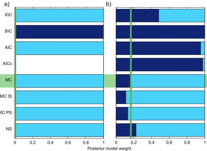
The overestimation or underestimation of BME itself might not be a major concern, if it yielded consistent results in model weighting, i.e., if the estimated BME values were correlated with the exact values, so that ratios of BME between alternative models were consistent. Furthermore, the AIC(c) is derived to assess dif-ferences between competing models, and one would expect to see a better approximation to the true model weights than to the absolute BME values. To investigate this, we determine the model ranking for the four models described in section 4.1. We further introduce two additional versions of the base case model L2 by using two different prior distributions: Model L2a (see Figure 2) acts on an informative prior which has a significant overlap with the area of high likelihood. Model L2b uses a slightly less informative prior, which is significantly shifted away from the area of high likelihood. Model L2a is therefore clearly the favorite among those two model versions, because it makes better predictions while being even more parsi-monious. We deliberately include those two versions as competing models to illustrate the inability of the AIC(c) and the BIC to detect differences in the parameter prior. We assign equal prior weights to all six mod-els to let BME be the decisive factor in model averaging (see equation (2)).
The AIC, AICc, and BIC assign a too large weight to the simplest model in the set (L1). This is due to the fact that these criteria merely count the number of parameters used by a model, instead of considering correla-tions among the parameters (defined by the parameter prior) which reduce the actual degrees of freedom. Furthermore, these criteria are not able to distinguish between the three models L2a, L2, and L2b, which only differ in their prior parameter assumptions, but not in their respective MLE. The corresponding BME approximations by AIC, AICc, and BIC therefore yield the most indecisive weighting for these three models (equal weights), whereas the true BMA weights convey the clear message that, out of these three models, L2a should be preferred over L2, and L2b should be discarded.
Within this model set, the nonlinear models obtain very small weights (see Figure 6) in the reference solu-tion because the model structure of NL2 does not match the data well and NL4 is already too complex to compete with the simpler linear models. Since the BME approximation errors of the KIC variants increase drastically with the nonlinearity of the models, these errors are expected to impact model ranking signifi-cantly if nonlinear models are playing a relevant role in the model selection competition. Here the nonlinear models play an almost irrelevant role and thus model ranking is not too badly compromised when using the KIC@MLE or the KIC@MAP, with the latter still outperforming the former.
4.7. Conclusions From Synthetic Test Case
The benchmarking has shown that all ICs (except for the KIC@MAP) potentially yield unacceptably large errors in BME approximation. Their performance depends on the actual data set (including the out-come of measurement error) that is used for calibration. We have learned that the AIC and AICc behave differently from the BIC and KIC for increasing data set size, i.e., the error made by the AIC(c) increases, while the error of the BIC and KIC decreases. Under varied prior information, however, the BIC follows the error behavior of the AIC(c) in that it cannot dis-tinguish models which only differ in their prior definition of the parameter space. This is a crucial finding, since the prior contains all the information about the Table 2.Relative Error of BME Approximation Methods for Different Model Structures as Compared to the Reference Solution (Analyti-cal Solution Equal to the KIC@MAP in Case of Linear Models, Brute-Force MC Integration in Case of Nonlinear Models, Highlighted in Italic Font)a
Method Erel;L1(%) Erel;L2(%) Erel;NL2(%) Erel;NL4(%)
KIC@MLE 0.9 30.4 24.9 99.8
KIC@MAP 0.0 0.0 13.2 59.4
BIC 94.0 21.3 37.5 70.3
AIC 176.4 59.7 179.2 22.5
AICc 137.0 3.2 69.4 83.4
MC 0.0 0.0 0.0 0.0
MC IS 0.8 [0.0; 2.2] 0.1 [0.0; 0.4] 1.1 [0.0; 2.9] 1.5 [0.1; 4.1] MC PS 132.0 [25.7; 196.6] 131.8 [23.5; 221.7] 324.8 [40.8; 490.3] 232.8 [18.1; 481.8] NS 2.4 [0.1; 6.4] 2.8 [0.4; 27.2] 4.0 [0.2; 10.7] 11.2 [3.3; 18.9]
a
95% Bayesian confidence intervals of numerical results given in parentheses.
0 0.2 0.4 0.6 0.8 1
NS MC PS MC/MC IS AICc AIC BIC KIC@MAP KIC@MLE
10-4 10-2 0
Posterior model weight
L1 L2a L2 L2b NL2 NL4