Decision Making in Networked Systems

(1)

University of Pennsylvania

ScholarlyCommons

Publicly Accessible Penn Dissertations

1-1-2015

Decision Making in Networked Systems

Mohammad Hadi Afrasiabi

University of Pennsylvania, [email protected]

Follow this and additional works at:

http://repository.upenn.edu/edissertations

Part of the

Engineering Commons

This paper is posted at ScholarlyCommons.http://repository.upenn.edu/edissertations/1574

For more information, please [email protected].

Recommended Citation

(2)

Decision Making in Networked Systems

Abstract

Living in a networked world, human agents are increasingly connected as advances in technology facilitates the flow of information between and the availability of services to them. Through this research, we look at interacting agents in networked environments, and explore how their decisions are influenced by other people's decisions. In this context, an individual's decision may be regarding a concrete action, e.g., adoption of a product or service that is offered, or simply shape her opinion about a subject. Accordingly, we investigate two classes of such problems.

The first problem is the dynamics of service adoption in networked environments, where one user's adoption decision, influences the adoption decision of other users by affecting (positively or negatively) the benefits that they derive from the service. We consider this problem in the context of "User-Provided Connectivity", or UPC. The service offers an alternative to traditional infrastructure-based communication services by allowing users to share their "home base" connectivity with other users, thereby increasing their access to connectivity. We investigate when such services are viable, and propose a number of pricing policies of different

complexities. The pricing policies exhibit differences in their ability to maximize the total welfare created by the service, and distributing the welfare between different stakeholders.

The second problem is the spread of opinions in a networked environment, where one agent's opinion about an issue, influences and is influenced by that of other agents to whom she is connected. We are particularly interested in the role that people's adherence to specific groups or parties may play in how final opinions are formed. We approach this problem using a model of interactions inspired by the Ising spin-glass model from classical Physics. We consider two related but distinct settings, and show that when party memberships directly influence user interactions, even slightest statistical partisan biases result in partisan final outcomes: where everyone in a party shares the same opinion, opposite to that of the other party. On the other hand, if party membership plays an indirect role in biasing agent interactions, then there is room for intra-party heterogeneity of opinions.

Degree Type

Dissertation

Degree Name

Doctor of Philosophy (PhD)

Graduate Group

Electrical & Systems Engineering

First Advisor

Roch Guerin

Keywords

(3)

Subject Categories

(4)

Decision Making in Networked Systems

Mohammad Hadi Afrasiabi

A DISSERTATION

in

Electrical and Systems Engineering

Presented to the Faculties of the University of Pennsylvania

in

Partial Fulfillment of the Requirements for the

Degree of Doctor of Philosophy

2015

Supervisor of Dissertation

Roch Gu´erin,

Harold B. and Adelaide G. Welge Professor of Comp. Sci, Washington U. in St. Louis

Graduate Group Chairperson

Saswati Sarkar,

Professor of Electrical and Systems Engineering

Dissertation Committee

Roch Gu´erin, Harold B. and Adelaide G. Welge Professor of Comp. Sci, Washington U. in St. Louis

Kartik Hosanagar, Professor of Internet Commerce, Wharton School of U. of Pennsylvania

Ali Jadbabaie, Alfred Fitler Moore Professor of Network Science, Elec. & Sys. Engineering

(5)

Decision Making in Networked Systems

This work is licensed under the Creative Commons Attribution-NonCommercial-ShareAlike 4.0 License. To view a copy of this license, visit

(6)

ACKNOWLEDGMENTS

I owe my deepest gratitude to my dissertation advisor and my mentor, Dr. Roch Gu´erin. Roch is a pioneer in the field of networking, a rigorous scientist and a visionary researcher,

and has been a dedicated teacher and an inspiring role model for me. I am grateful for

hav-ing his unreserved help, continuous guidance, and insightful recommendations throughout my PhD studies at Penn.

I would like to sincerely thank Dr. Santosh Venkatesh, my dissertation committee chair,

for his generous support and his valuable lessons. I am also thankful to my dissertation committee members, Dr. Kartik Hosanagar and Dr. Ali Jadbabaie, for their time and for

kindly offering me their advice.

I thank the National Science Foundation for supporting my research. This dissertation would not have been possible without funding from them.

I warmly thank my parents, Hassan and Banoo, for their selflessness, and for believing

in their children, and for always encouraging their children to the pursuit of knowledge. I also thank my siblings, Elham, Somaieh, Maryam and Mohammad Reza.

My last and most special thanks to my fianc´e, Golnar, for her love and her support, and

(7)

ABSTRACT

Decision Making in Networked Systems

Roch Gu´erin

Living in a networked world, human agents are increasingly connected as advances in technology facilitates the flow of information between and the availability of services to

them. Through this research, we look at interacting agents in networked environments,

and explore how their decisions are influenced by other people’s decisions. In this context, an individual’s decision may be regarding a concrete action, e.g., adoption of a product

or service that is offered, or simply shape her opinion about a subject. Accordingly, we

investigate two classes of such problems. The first problem is the dynamics of service adoption in networked environments, where one user’s adoption decision, influences the

adoption decision of other users by affecting (positively or negatively) the benefits that

they derive from the service. We consider this problem in the context of “User-Provided Connectivity”, or UPC. The service offers an alternative to traditional infrastructure-based

communication services by allowing users to share their “home base” connectivity with other

users, thereby increasing their access to connectivity. We investigate when such services are viable, and propose a number of pricing policies of different complexities. The pricing

policies exhibit differences in their ability to maximize the total welfare created by the

service, and distributing the welfare between different stakeholders. The second problem is the spread of opinions in a networked environment, where one agent’s opinion about an

issue, influences and is influenced by that of other agents to whom she is connected. We are particularly interested in the role that people’s adherence to specific groups or parties

may play in how final opinions are formed. We approach this problem using a model of

interactions inspired by the Ising spin-glass model from classical Physics. We consider two related but distinct settings, and show that when party memberships directly influence

user interactions, even slightest statistical partisan biases result in partisan final outcomes:

where everyone in a party shares the same opinion, opposite to that of the other party. On the other hand, if party membership plays an indirect role in biasing agent interactions,

(8)

Chapter 1 Introduction

Individuals1 living in the networked modern world interact with each other in a variety of

ways. They consume and share information, goods and services, whereby influencing each

other’s decisions and behaviors [33]. These interactions complicate the decision-making

patterns in networked settings, and there has been growing interest in understanding and

predicting such patterns [28,35,36], which require consideration of how individuals perceive

and react to external influences, or “externalities”.

The concept of externalities (also called “network effect”) has been traditionally used

for modeling the adoption of goods and services in networked settings [27]. A product

with positive externalities, for example, is one that becomes more appealing as more people

use it. In this research, we study2 various problems in networked settings where individuals

face complex positive and negative externalities, and investigate how the tug of war between

different types of externalities shapes individuals’ decisions and behaviors in those settings.

In this context, an individual’s decision may be regarding a concrete action,e.g., adoption

of a new product or service that is offered, or simply shape her opinion regarding a subject.

In both cases, the person’s decision includes a component that is contributed by others.

Accordingly, we investigate two classes of such problems.

1_{We may use the terms “individual”, “person” and “agent” interchangeably to refer to an entity in a}

networked setting, as may be represented by a “node” in the network’s graph.

2 _{This dissertation is based on work with Roch Gu´}_{erin and Santosh Venkatesh, parts of which has}

(13)

The first problem is the dynamics of service adoption in networked environments, where

one user’s adoption decision influences the adoption decisions of other users by affecting

(positively or negatively) the benefits that they derive from the service. We consider this

problem in the context of “User-Provided Connectivity, or UPC, which we introduce in

Section1.1 with full investigation given in Chapter3.

The second problem is the spread of opinions in networked environments, where one

agent’s opinion about an issue, influences and is influenced by that of other agents to whom

she is connected. We are particularly interested in the role that people’s adherence to

specific groups or parties may play in how final opinions are formed. We introduce this

problem in Section1.2, with full investigation provided in Chapter4.

In Chapter 2we review the related work in this area.

1.1 Adoption of service in user-provided connectivity

Network services often exhibit positive and negative externalities that affect users’ adoption

decisions. One such service is “user-provided connectivity” or UPC. The service offers an

alternative to traditional infrastructure-based communication services by allowing users to

share their “home base” connectivity (see [64] for an example) with other users, thereby

increasing their access to connectivity.

More users mean more connectivity alternatives, i.e., a positive externality, but also

greater odds of having to share one’s own connectivity,i.e.,a negative externality. The tug

of war between positive and negative externalities together with the fact that they often

depend not just on how many but also which users adopt, make it difficult to predict the

service’s eventual success. We explore this issue, and investigate not only when and why

such services may be viable, but also explore how pricing can be used to effectively and

practically realize them.

Towards this goal, we develop a simple model that helps understand how the different

factors interact and affect the adoption of a UPC service and the total welfare (sum of users’

(14)

between users and the service provider. To maintain analytical tractability, the model makes

a series of simplifying assumptions, many of which may arguably not hold in practice.

However, the analysis affords insight that, as we demonstrate, remains valid even under

more general settings. Specifically, our main contributions consist of

• Formulating and solving a simple model that captures key features of a UPC type of

service;

• Characterizing when and how the service’s total welfare, or value, is maximized;

• Identifying practical pricing policies that realize a different trade-off between

optimiz-ing welfare and distributoptimiz-ing it between stakeholders.

• Numerically validating the robustness of the findings, when relaxing the simplifying

assumptions on which the model relies.

1.2 Opinion formation in biased networks

Social interactions commonly take place in a networked setting where an individual’s opinion

is influenced by the opinions of others. We allow this influence to be positive or negative,

biased by partisan affiliations of connected individuals. Such signed influences are akin to

the positive and negative externalities described earlier for the adoption of a UPC service.

Our work explores the role of partisan influence in the emergence of consensus opinions in

social network settings.

We study a network of nodes where each node holds an opinion — a binary state that

may update over time under the influence of a node’s neighbors. Nodes have biased affinities,

which logically partition the network into distinct parties. Nodes in the same party tend

to have a positive influence on each other, but the extent to which this holds varies across

nodes and depends on the chosen affinity model.

We consider two variations on an Ising spin-glass network model (from classical physics)

that investigate opinion formation in such biased affinity systems. These models differ in

(15)

The first of these in what we term the random influence model randomly selects the

influence two nodes exert on each other based on their respective party affiliation. The

second, a profile-based model, relies on a profile, a κ-bit vector of ±1 entries based on the

node’s known positions regarding each ofκindependent topics. In this model the similarity

of the profiles of two nodes determines whether they have a positive or negative influence

on each other’s opinions.

We investigate the formation of opinions under both models and characterize their fixed

points (equilibria). We show that while these systems always converge to a fixed point,

they differ in their number and types of fixed points. Under a direct party impact as in

the random influence model, opinions nearly always converge to a partisan outcome with

parties settling on unanimous, antagonistic positions. In the profile-based model, the shift

from a direct to an indirect role in how party affiliation impacts decisions translates into

significant differences in the type of outcomes that can arise. In particular, party unanimity

is not the norm anymore.

While we initially assume that all nodes are connected (full graph) and also that all

nodes are members of one of two parties, with nodes from the same party more likely to

exhibit a positive affinity bias, we later relax these assumption. Specifically, we introduce

two set of modifications to our models. We first study the effect of a third group of nodes,

e.g., independent nodes who have unbiased affinities towards other nodes, irrespective of

party affiliations. We then consider the impact of additional structure, in the form of an

Erd˝os-R´enyi graph (as opposed to a full graph), that determines which nodes interact with

(16)

Chapter 2 Related works

The types of problems described in Chapter 1, that exhibit interconnected agents and

mutual interactions, belong to a broader set of questions that naturally emerge in networked

settings and have become prevalent in many different areas,e.g., economics, social science,

biology, engineering and political science. The growing importance of, and interest in, such

questions is behind the emergence of “Network Science” as a new independent field [27,33,

50,76].

The breadth of topics that network science spans also means that multi-disciplinary

approaches are typically needed when tackling problems [37,47,68]. This is well illustrated

in our work, which relies on techniques from marketing research and statistical physics to

tackle the problems of service adoption and opinion formation in the presence of party biases

that it is concerned with. Similarly, researchers from seemingly disparate backgrounds have

contributed to the field of network science. In the past decade, a number of books have

aggregated the various studies in this field [33,51,54,72,90]. Such books provide a thorough

review of the different techniques for study of network systems, as well as their implications

and predictions.

In the next two sections we provide a more specific review of the literature as related to

the particular problems that we study, namely, where the “externalities” play a prominent

(17)

2.1 Adoption of products and services

The service adoption process that we introduce in Chapter 3 involves settings that are

studied under the umbrella of systems theory and/or game theory in various fields, from

engineering [8,13,46,83] to economics [9]. In the language of the latter, our work considers

a forward looking monopolistic service provider who tries to optimally price a service and

offers it to a set of heterogeneous myopic users, who in turn play a best-response dynamics

game until the system potentially reaches a pure-strategy Nash equilibrium.

Best-response dynamics [41] in game theory refers to scenarios where agents repeatedly

improve their choice until a Nash equilibrium is reached. Such a procedure provides a

plausible path to realizing a Nash equilibrium of the system, whence the agents are said

to “learn the equilibrium” [78]. Learning in game theory is also considered in [40], and is

closely related to the subjects ofpotential games[14,69] and evolutionary game theory [87].

Another related area in game theory consists of the works on the concept of “price of

anarchy” [59], which is similar in flavor to our discussion in Section 3.7.3 on sub-optimal

welfare realization.

In studying systems with heterogeneous users and in the presence of externalities, it

is common [7,21,25,81] to assume some knowledge of the state of the system, e.g., users’

characteristics, or ”types”, for the other users and the provider. For instance, [25] assumes

that the monopolist has complete knowledge of the graph structure and therefore is able to

measure the individual network characteristics of each user. Similarly, [7] assumes that the

seller knows the probability distribution for the users’ valuation of the good, and that the

knowledge of the state of the system can propagate to users. In our analytical models too,

we assume that while the provider does not have knowledge of the individual user types,

it knows their probability distribution1. We also assume that users know the state of the

system, as the level of adoption and the type of current adopters can be inferred by a user

by observing the available service coverage and the roaming traffic that goes through one’s

1

(18)

home base. As such, our models represent a game with “incomplete information”, since

while the distribution of users’ utility function is known, individual users’ utilities are not.

Also, users have “perfect information”, in that they know the moves previously made by

all other players.

An important property of the adoption models that we introduce is that they exhibit

both positive and negative externalities. There is a vast literature investigating the effect of

externalities, often callednetwork effects [34,62,63], but the majority of these works focus on

either positive or negative externalities separately. For example, [24] investigates the impact

of positive externalities on the product adoption decisions of individuals. The effect of

positive externalities on the competition between technologies is considered in [39,55,56] and

extended to include converters and switching costs in several other works,e.g.,[30,38,53,82].

Conversely, the impact of negative externalities,e.g., from congestion, has been extensively

investigated in the context of pricing for both communication networks [43,57,66,75,85]

and transportation systems [16,23,58,73].

The topic of optimal pricing for systems with both positive and negative externalities is

less studied and seems to have been first addressed in [29] that sought to optimize a

com-bination of provider’s profit and consumers’ surplus. Different pricing strategies were

con-sidered, including flat pricing and pricing strategies that account for the product “amount”

consumed by a user,i.e.,akin to the usage-based pricing model of Section3.5. Other works

have been primarily conducted in the context of the theory of clubs first formally introduced

in [22] (see [10,77,80] for more recent discussions). A club has a membership that shares

a common good or facility, e.g., a swimming pool, so that increases in membership have

a positive effect (externality) by lowering the cost share of the common good, e.g., lower

maintenance costs of the shared swimming pool. At the same time, a larger membership also

has a negative, congestion-like effect,e.g., a more crowded swimming pool. In general, the

co-existence of positive and negative externalities implies an optimal membership size (see

also [52] for a recent interesting investigation that contrasts the outcomes of self-forming

(19)

Club-like behaviors also manifest themselves in file-sharing peer-to-peer (p2p) systems.

In a file-sharing p2p system, more peers increase the total resources available to store

content. However, unless enough peers are willing to share their resources, more peers can

also translate into a higher load on those peers willing to serve files to others, and/or a

longer time for locating a desired file. This has then triggered the investigation ofincentive

mechanisms to ensure that enough peers share their resources,e.g.,BitTorrent “tit-for-tat”

mechanism [31] or [32] that also explores a possible application to a wireless access system

similar in principle to the one we consider in Chapter3.

Our model differs from these earlier works in important ways. First and foremost, it

in-troduces a model for individual adoption decisions of a service, which allows for

heterogene-ity in the users’ valuation of the service. In particular, certain users (roaming users) have a

strong disincentive to adoption when coverage/penetration is low, while others (sedentary

users) are mostly insensitive to this factor. Conversely, this heterogeneity is also present in

the negative externality associated with an increase in service adoption. Its magnitude is

a function of not just the number of adopters, but their identity as well, i.e., roaming or

sedentary users. The presence of heterogeneity in how users value the service and how they

affect its value is a key aspect of a UPC–like service; one that influences its value and how

to price it to realize this value.

2.2 Formation and spread of opinions

Tools from statistical physics have been adapted for use in economics, models of neural

computation, as well as to offer models of social interactions in network settings [15,20,

71,74]. In the latter setting, the phenomenon of community structure in social networks

and graphs has seen some attention in the literature. Community structure refers to the

presence of modular groups in networks where individual members inside a community are

highly connected but connections between members of different communities are sparse or

non-existent. In particular, members of any one community exert little or no influence on

(20)

Works in this area include [44], which uses centrality indices in graphs to detect

com-munity structure, [18] which identifies mechanisms to generate networks with community

structure, and [60] which studies the formation of opinions in these settings.

These works reflect the tendency of individuals in a society to assemble in smaller groups

that are not necessarily connected. They do not, however, capture partisan interactions

between parts of a society, where individuals from different groups co-mingle and interact

in a manner shaped by their respective party or group, in the process exerting positive and

negative influences on each other.

Various models of positive and negative interactions in a spin glass framework have also

been considered in the literature [15,19]. In these settings agents are considered to be

sta-tistically exchangeable with noa priori biases in the strengths of their random interactions

with other agents. These models lead to the characteristic disorder-induced phase

transi-tions of spin glass models but do not in themselves make provision for partisan behaviour

in opinion formation.

A variety of other models of opinion formation in sociological settings have been

con-sidered in the literature. These include the energy-driven Ising spin glass model, the voter

model, the Szanjd model, and the bounded-confidence model [17,26,65,67,79,86]. These

models all feature agents influencing each other’s opinions in a number of different ways.

While the posited mechanisms vary, agent interactions in these models area priori unbiased

and their influence on each other is only through the prism of their opinions; there is no

party or group structure influencing interactions. As we shall see in Chapter 4,

fundamen-tally different behaviours arise when interactions are influenced, however slightly, by an

(21)

Chapter 3 User-Provided Connectivity

3.1 Introduction

There is no denying that we are a networked society, and many networked goods or services

exhibit strongexternalities,i.e.,a change — positive or negative — in the value of one unit

of good, as more people use those goods. For example, Metcalfe’s law [27, p.71] captures

the positive effect on a network value of having more users, while the increased congestion

that arises from the added traffic contributes a negative externality. Externalities, and

more generally the benefits derived from goods or services, vary across users, i.e., exhibit

heterogeneity. This makes predicting the impact of externalities difficult, especially when

positive and negative forces interact. A basic question of interest is then to determine

(ahead of time) if and how offerings of goods or services that exhibit positive and negative

externalities will succeed or fail.

The original motivation for this work was answering this question for a specific service,

namely,user provided connectivity or UPC. The goal of UPC is to address the rising thirst

for ubiquitous data connectivity fueled by the fast growing number of capable and versatile

mobile devices. This growth has taxed the communication infrastructure of wireless carriers

to the point where it is threatening their continued success [91]. Addressing this issue

(22)

for “off-loading” some of the traffic. WiFi off-load solutions (e.g., as embodied in the

Hotspot2.0 initiative of the WiFi Alliance and the Next Generation Hotspot (NGH) of

the Wireless Broadband Alliance) offer a possible option, of which FON1 demonstrated a

possible realization. FON users purchase an access router (FONERA) that they use for

their own local broadband access, but with the agreement that a (small) fraction of their

access bandwidth can be made available to other FON users. In exchange, they receive the

same privilege2 _{when roaming,} _i.e., _{can connect through the access points of other FON}

users.

Under a UPC scheme, connectivity grows “organically” as more users join the network

and improve its coverage, and the challenge is to determine if it can reach sufficient critical

mass to be viable. Consider for example a FON-like service starting with no users. This

makes the service unattractive to users that value ubiquitous connectivity highly,e.g.,users

that roam frequently, because the limited coverage offers little connectivity beyond that of a

user’s “home base”. On the other hand, sedentary users are mostly insensitive to the initial

minimal coverage, and if the price is low enough can derive positive utility from the service;

hence join. If enough such (sedentary) users join, coverage may increase past a point where

it becomes attractive to roaming users who will start joining. This would then ensure rapid

growth of the service, were it not for a negative dimension to that growth.

Specifically, as more roaming users join, they compete for connectivity and may

en-counter increasingly congested access points. Conversely, sedentary users end-up having to

share their home access more frequently. This may be sufficient to convince them to drop

the service (unlike roaming users, they do not see much added value from the better

cov-erage). The resulting reduction in coverage would in turn affect roaming users, who could

then also start leaving. Hence, after an initial period of growth, the service may experience

a decline.

The extent to which such behaviors arise depends on many factors, and in particular

1

http://www.fon.com. See also AnyFi (www.anyfinetworks.com) or previously KeyWifi, and also more recently Comcast [64] for similarly inspired services.

2

(23)

the trade-off between service cost and users’ sensitivity to the positive and negative aspects

of a growing user-base. Making the service “free” would clearly maximize adoption, but

unless other revenue sources are available, e.g., ads, is unlikely to allow it to be viable.

Increasing the service price could affect (lower) adoption, but may improve its viability.

More generally, service pricing offers a “control knob” that can be used to realize a variety

of objectives,e.g.,maximizing overall value or welfare, or maximizing provider’s profit, etc.

This control knob can be complex and involve offering the service at a different price to

each user, i.e., discriminatory pricing [11], or very basic, e.g., fixed pricing, and there is

typically a trade-off between how well objectives can be met and the complexity of the

control (pricing) used to meet them.

In this chapter we develop a simple model that helps understand how these factors

interact and affect the adoption of a UPC service and the welfare (sum of users’ utility

and provider’s profit) it creates, and how that welfare can be efficiently distributed between

users and the service provider. To maintain analytical tractability, the model makes a series

of simplifying assumptions, many of which may arguably not hold in practice. However,

the analysis affords insight that, as we demonstrate, remains valid even under more general

settings. Specifically, this chapter’s main contributions consist of

• Formulating and solving a simple model that captures key features of a UPC type of

service;

• Characterizing when and how the service’s total welfare, or value, is maximized;

• Identifying practical pricing policies that realize a different trade-off between

optimiz-ing welfare and distributoptimiz-ing it between stakeholders.

• Numerically validating the robustness of the findings, when relaxing the simplifying

assumptions on which the model relies.

The rest of the chapter is structured as follows. Section 3.2 presents the model we

rely on to capture the properties of a UPC service. Section 3.3 explores when and how

the service value (total welfare) is maximized. Section 3.4introduces the role of pricing in

(24)

policies, i.e.,usage-based (Section 3.5), hybrid (Section3.6), and fixed-price (Section 3.7).

Section 3.9 discusses generalizations and robustness of the findings. A summary of the

chapter’s findings is provided in Section 3.10.

3.2 Model Formulation

This section introduces a model that captures key aspects of adoption of a UPC-like service

by users. We first present the general form of the model in Section 3.2.1. We then

intro-duce a series of simplifying assumptions in Section 3.2.2to obtain a simpler model that is

analytically tractable. Verifying that the findings afforded by this simplified model remain

valid in more general situations calls for a two-prong approach: (1) An explicit solution is

developed that offers a qualitative understanding of and insight into what drives the success

(or failure) of UPC systems; (2) The robustness of those findings is then numerically tested

under configurations that emulate more general settings,i.e.,where the model’s simplifying

assumptions are relaxed and errors are present in the estimation of its parameters.

3.2.1 General form

Given the expected organic growth of a UPC service, the interplay between the coverage

it realizes and its ability to attract more users is of primary interest. The service coverage

κ depends on the level x of adoption in the target user population, and determines the

odds that users can obtain connectivity through the service while roaming. Users are

heterogeneous in their propensity to roam, as captured through a variableθ,0≤θ≤1. A

user’s exact θ value is private information, but its distribution (over the user population)

is known. A low θ indicates a sedentary user while a high θ corresponds to a user that

frequently roams. Hence,θ determines a user’s sensitivity to service coverage.

As commonly done [24], a user’s service adoption decision is based on the utility she

derives from the service; she decides to adopt if that utility is positive. A user’s utility is

(25)

the current set of adopters. The general form of U(Θ, θ) is given in Eq. (3.1).

U(Θ, θ) =F(θ, κ) +G(θ, m)−p(Θ, θ), (3.1)

wherem is the volume of roaming traffic generated3 by the current set of adopters Θ.

F(θ, κ) reflects the overall utility of connectivity, either at home or roaming, while

G(θ, m) accounts for the negative impact of roaming traffic. Finally, p(Θ, θ) is the price

charged to the userθ when the adopters’ set is Θ.

Note that the price p(Θ, θ) is a control parameter that affects service adoption,i.e., it

can be endogenized to achieve specific objectives. In this chapter, we explore the use of

pricing to maximize total welfare and/or profit. Other parameters are exogenous and can

be estimated, e.g., using techniques from marketing research as discussed in [45], but not

controlled.

Building on Eq. (3.1), users adopt the service only if their utility is positive, and are

myopic when evaluating the utility they expect to derive from the service,i.e.,they do not

anticipate the impact of their own decision on other users’ adoption decisions. However,

adoption levels affect coverage, and as coverage changes, so does an individual user’s utility

and, therefore, her adoption decision.

The level of adoption x is given by

x=|Θ|_, Z

θ∈Θ

f(θ)dθ,

wheref(θ) is a density function and reflects the distribution of roaming characteristics over

the user population.

In the next section, we specialize the different terms in the utility function of Eq. (3.1).

3

(26)

3.2.2 Assumptions and the simplified model

For analytical tractability, we make several assumptions regarding the form and range of

the parameters of Eq. (3.1) (Section3.9explores the impact of relaxing these assumptions).

First, a user’s propensity to roam, as measured byθ, is taken to be uniformly distributed

in [0,1], i.e.,

f(θ) = 1, 0≤θ≤1.

This implies that given a set of adopters Θ, the adoption level,x is

x= Z

θ∈Θ

dθ . (3.2)

Conversely, assuming that every user contributes one unit of traffic, the volume of roaming

trafficm generated by current adopters is given by

m= Z

θ∈Θ

θ dθ . (3.3)

Next, we assume that the distributions of users over the service area and their roaming

patterns are uniform. A uniform distribution of users implies that the adoption levelx also

measures the availability of connectivity to roaming users, henceκ=x. Similarly, uniform

roaming patterns mean that roaming users (and traffic) are evenly distributed across users’

home bases,i.e., all see the same connectivity while roaming. Therefore, we can write the

functionF(θ, κ) as

F(θ, κ) = (1−θ)γ+θ rx . (3.4)

The parameter γ ≥0 measures the utility of basic home connectivity, while r ≥0 reflects

the utility of roaming connectivity.4 The latter needs to be weighed by the ”odds” that

such connectivity is available, which are proportional to the current service coverageκ=x.

Hence,rx is the (true) utility of roaming connectivity, when the level of coverage isκ=x.

4

(27)

The additional factors 1−θ and θ in Eq. (3.4) capture the impact of a user’s roaming

characteristic in how it uses, and therefore values, home and roaming connectivity.

Specif-ically, a user with roaming characteristicθ splits its connectivity time in the proportionsθ

and 1−θ between roaming and home connectivity, respectively.

Further, the impact of roaming traffic is assumed proportional to its volume m, which

based on the assumption of uniform roaming patterns, is equally distributed across adopters’

home bases. Specifically, the (negative) utility associated with roaming traffic consuming

resources in the home base of users is proportional to −cm , c ≥0. Roaming traffic affects

equally the users whose home base it uses, and the roaming users seeking connectivity

through it. Hence, all users experience the same impact of the form −θcm−(1−θ)cm=

−cm, so that G(θ, m) is5

G(m) =−c m .

Under these assumptions, a user’s utility is of the form

U(Θ, θ) =γ−c m+θ(r x−γ)−p(Θ, θ). (3.5)

In the next section, we characterize the total welfare that can be created by a UPC

service as a function of the service parameters (exogenous and endogenous).

3.3 Total Welfare

In this section, we characterize the total welfare (value) a UPC service can create for

its adopters and provider. Adopters’ welfare is through the utility they derive from the

service, while the provider’s welfare is from what it charges adopters for the service. Using

the model introduced in the previous section, we derive analytical conditions under which

the total welfare is maximized. As argued earlier, the benefit of such analytical solutions

is in providing insight into when and why the service may be valuable (worth deploying).

5

(28)

The validity of that insight is tested under more general conditions in Section 3.9.

To compute the maximum welfare, we first obtain the optimal set of adopters Θ∗(x) for

any given adoption levelx, and then solve for the optimal x.

3.3.1 Optimal Adoption Set for Given Adoption Level

For a given adoption levelx, we seek the set of adopters Θ,|Θ|=x,that maximizes welfare.

Provider’s welfare (or profit) WP can be written as

WP(Θ) = Z

θ∈Θ

(p(Θ, θ)−e) dθ , (3.6)

wherep(Θ, θ) is the price charged to a user with roaming characteristic θgiven a set Θ of

existing adopters, and eis the per customer cost of providing the service, e.g., as incurred

from billing, customer service, or equipment cost subsidies6. Conversely users’ welfare is

given by

WU(Θ) = Z

θ∈Θ

U(Θ, θ)dθ . (3.7)

The service welfare,V(Θ), is the sum of these two quantities.

V(Θ) =WU(Θ) +WP(Θ)

= Z

θ∈Θ

U(Θ, θ) +p(Θ, θ)−e

dθ.

(3.8)

For notational purposes, we denote the integrand in Eq. (3.8) by v(Θ, θ),

v(Θ, θ),U(Θ, θ) +p(Θ, θ)−e ,

which can be interpreted as theindividual value adopterθcontributes to the service. Using

6_{Note that this cost is ultimately born by the users, as it affects the price the provider charges for the}

(29)

Eq. (3.5) we can rewrite Eq. (3.8) as

V(Θ) = Z

θ∈Θ

γ+θ(rx−γ)−cm−e

dθ. (3.9)

Characterizing optimal welfare for a given adoption levelx, therefore calls for identifying

the set Θ∗(x) of adopters of cardinalityx,|Θ∗|=x, which maximizes Eq. (3.9). This is the

subject of the next lemma, which is proved in AppendixA.9 in a more general form.

Lemma 1. For any adoption level x, maximum welfare is always obtained with a set of

adoptersΘ∗(x) that exhibit contiguous roaming characteristics. Specifically,Θ∗(x) is of the

form

Θ∗(x) =       

Θ∗₁(x) = [0, x) ifx < _r₋γ_c,

Θ∗₂(x) = [1−x,1] ifx≥ _r₋γ_c.

(3.10)

3.3.2 Optimal Adoption Level

From Lemma1, we obtain the optimal welfareV∗(x),V(Θ∗(x)) given any adoption level

x. Following the partition of Eq. (3.10) into two cases x ∈ [0, _r₋γ_c) and x ∈ [_r₋γ_c,1], we

consider separately the cases of V(Θ∗₁(x)) andV (Θ∗₂(x)).

Using Eq. (3.10) in Eq. (3.3) gives forx∈[0, _r₋γ_c),

m(Θ∗₁(x)) = Z x

θ=0

θdθ = x 2

2 ,

and therefore by and Eq. (3.9)

V(Θ∗₁(x)) = r−c

2 x

3₋ γ 2x

2_{+ (}_γ₋_e₎_x.

Similarly, for x∈[_r₋γ_c,1], the roaming traffic corresponding to Θ∗₂(x) is

m(Θ∗₂(x)) = Z 1

θ=1−x

θdθ= 1

2 2x−x 2

(30)

and therefore by Eq. (3.9)

V(Θ∗₂(x)) =−r−c

2 x

3_{+ (}γ

2 +r−c)x 2₋_ex.

Combining the above expressions, the optimal service valueV∗(x),V(Θ∗(x)) for a given

adoption levelx is given by

V∗(x) =    

  

r−c

2 x

3₋ γ 2x

2_{+ (}_γ ₋_e₎_x _if_{x <} γ r−c

−r−₂cx3+ (γ₂ +r−c)x2−ex ifx≥ _r₋γ_c,

where Θ∗(x) andx are related by Eq. (3.10).

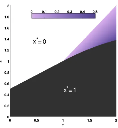
Given V∗(x), we can then solve for the valuex∗ that maximizes V∗(x). The

computa-tions are mechanical in nature and are given in Appendix A.2, with Fig.3.1illustrating x∗

as a function ofγ and e(for r−c= 1).

The solution can be partitioned into two different regimes based on the value ofγ. When

γ ≤r−c(corresponding to γ≤1 in Fig.3.1), optimal adoption is eitherx∗= 1 or x∗ = 0,

depending on the service cost e. If the service cost is low (e < γ+r₂−c), then maximum

welfare occurs forx∗ = 1, and it is

V∗(x= 1) = γ+r−c

2 −e. (3.11)

Conversely, if the service cost is high (e ≥ γ+r₂−c), then it overshadows any benefit or

utility the service produces and it is impossible to create positive welfare. In this case, the

“optimal” adoption isx∗ = 0.

In contrast, when γ > r−c (corresponding to γ > 1 in Fig. 3.1), intermediate values

0 < x∗ < 1 are possible (the gradient-shaded region of Fig. 3.1). This is because as γ

increases, sedentary users start to derive more utility and progressively become the dominant

value contributors. Therefore a set of (mostly) sedentary adopters can make a large positive

(31)

traffic, the optimal adoption level discourages frequently roaming users. Note that r −c

gives a tentative measure of the “net” importance of roaming (roaming utility factor less

roaming traffic factor), and as such the condition γ > r−cdescribes a system where home

connectivity has a higher value than the overall (“net”) effect of roaming connectivity. Such

a system may arguably not be a prime candidate for UPC services.

In summary, the main finding that emerges from the results of this section is that when

a UPC service can generate significant positive value, that value is typically maximized at

full adoption (or close to full adoption7) Section3.9 numerically tests the validity of this

finding when the model’s assumptions are relaxed.

While this section explored the relationship between service adoption and total welfare,

and identified adoption sets that maximize total welfare, the next section focuses on how to

realize such outcomes. As we shall see, this greatly depends on the flexibility of the pricing

policy used.

3.4 Role of Pricing

The analysis of Section 3.3 characterizes maximum service welfare, but does not offer a

constructive method to realize it. As shown in Eq. (3.5), adoption and, therefore, welfare,

depend onp(Θ, θ). Hence, maximizing welfare calls for identifying a suitablepricing policy.

Moreover, the pricep(Θ, θ) is also the parameter that determines how welfare is divided

between users and the provider. For example, if p(Θ, θ) = e, then the provider is only

compensated for its expensese (its profit is WP(Θ) = 0) and the entire welfare is realized

as user’s utility, WU(Θ) =V(Θ). Conversely, if p(Θ, θ) =v(Θ, θ) +e, then U(Θ, θ) = 0,

i.e.,users derive zero utility (strictly speaking, prices would be set to ensure an infinitesimal

but positive utility) and all of the welfare is realized as provider’s profit,WP(Θ) =V(Θ).

Other pricing schemes are possible that distribute welfare between users and the provider.

7

(32)

Figure 3.1: Regions of optimal adoption for maximum system value. Parameters arer = 1.6 andc= 0.6 (and thereforer−c= 1). The gradient-shaded area corresponds to 0< x∗ <1, whereas the solid black and white areas correspond to x∗ = 1 and x∗ = 0, respectively.

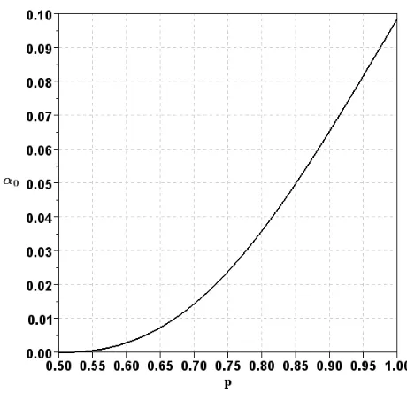
(a)θ0= 0 (b)θ0= 0.4 (c)θ0= 1

Figure 3.2: System value contributed by user θ0 as a function of x. Parameters are γ = 0.8, e= 0, c= 0.6, b= 0, r = 1.6.

For example, a price of the form

p(Θ, θ) =v(Θ, θ) +e−δ

= (1−θ)γ+θrx−cm−δ ,

(3.12)

(33)

(a)x= 0.2 (b)x= 0.5 (c)x= 1

Figure 3.3: System value contribution across users, at different adoption levels. Parameters areγ = 0.8, e= 0, c= 0.6, b= 0, r= 1.6.

utility U(Θ, θ) = δ > 0, hence realizing the optimal adoption level8 x = 1. Therefore,

the optimal welfare V∗(1) of Eq. (3.11) is realized and by usingU([0,1], θ) in Eq. (3.7) it

follows that the users’ overall welfare is

WU([0,1]) =δ .

This means that without affecting adoption, we can pick anyδ >0 to freely varyWU([0,1])

in the range (0, V∗(1)], and accordingly by Eq. (3.8),

WP([0,1]) =V∗(1)−WU([0,1]). (3.13)

In short, this policy realizes two important goals

• Optimal welfare, and

• Flexible welfare distribution.

Such a discriminatory pricing policy is, however, difficult to implement in practice as it

requires knowledge of individual user characteristics (θ) that may not be readily available9,

8

When optimal adoption is not atx= 1, optimal welfare can still be realized by setting a high price for users who should not adopt.

9

(34)

and also results in a price that varies with the adoption levelx. This heterogeneity across

both users and adoption levels is illustrated in Figs. 3.2 and 3.3, that plot v(Θ, θ) as a

function of θand x.

In the following sections, we introduce pricing policies that offer a different trade-off

between realizing maximum welfare, distributing it arbitrarily, and practicality.

3.5 Usage-based Pricing Policy

As mentioned above, a discriminatory pricing policy can both maximize total welfare and

distribute it arbitrarily between users and the provider. It is, however, difficult to implement

in practice. This section proposes a usage-based pricing scheme that mimics the behavior

of the discriminatory policy, but makes it feasible in practice. Under a usage-based pricing

scheme, users are charged based on how often they connect at home and while roaming. We

present next the structure of usage-based pricing, how it is able to capture key aspects of

discriminatory pricing, and also the insight that the analysis of the pricing policy affords.

3.5.1 Pricing Structure

In a UPC service, usage has two components,home usage denoted byzh,androaming usage

denoted byzr. A usage-based pricing policy may assign different prices to these two usage

types. Assuming that ph and pr are unit prices for home and roaming usage, respectively,

a user is charged

pz(zh, zr) =zh·ph+zr·pr−a, (3.14)

whereacorresponds to fixed usage allowance that may be given to each user, e.g., akin to

the free minutes commonly included in cellular phone plans.

Eq. (3.14) states what a user pays for the service as a function of her usage. Next,

we express this cost in terms of the user and service model of Section 3.2. This calls for

characterizing how roaming characteristicsθand the service coveragexaffect a user’s home

(35)

By definition, θ denotes a user’s propensity to roam, i.e., how often she is roaming

versus at home. However, because a roaming user successfully connects only where there is

coverage, her “typical” roaming usage is only zr(x, θ) =θx. Conversely, her typical home

usage is simply zh(θ) = 1−θ (home connectivity is always available). Replacing zh and

zr in Eq. (3.14) by the typical roaming and home usages zr(x, θ) and zh(θ) of a user with

roaming characteristics θ, we obtain the following expression for what she will typically be

charged for using a UPC service with a coverage level of x

p_z(x, θ) =ph(1−θ) +prθx−a. (3.15)

Eq. (3.15) has three parameters ph, pr and athat affect service adoption, i.e.,which users

derive positive utility. Given our goal of emulating the discriminatory pricing policy of

Eq. (3.12) and by comparing it to Eq. (3.15), we choose ph = γ and pr =r, which yields

the following usage-based pricing scheme

p_z(x, θ) =γ(1−θ) +rθx−a. (3.16)

We note that the only difference between Eq. (3.16) and the discriminatory pricing of

Eq. (3.12) is in the terms a versus cm−δ, where the former is constant while the latter

depends on the level of roaming trafficm. As we shall see next, this difference is minor, and

the usage-based pricing policy of Eq. (3.16) is capable of realizing both maximum welfare

and flexibility in how welfare is distributed across users and the provider.

3.5.2 Maximal Service Adoption

Using Eq. (3.16) in Eq. (3.5) gives the following expression for the utility derived by userθ

from adopting the service

(36)

We next use Eq. (3.17) to identify the adoption equilibria under usage-based pricing. We

say a set of adopters Θ comprises an equilibrium when

U(Θ, θ)>0, if θ∈Θ, and

U(Θ, θ)≤0, if θ6∈Θ.

Then,

Proposition 1. Under the usage-based pricing policy of Eq. (3.16), full adoption, x= 1,

is the unique equilibrium ifa > c/2, and is not an equilibrium if a≤c/2.

Proof. Recall that c ≥ 0, and note that at any adoption level x (corresponding to an

adopters’ set Θ such that |Θ| = x), the roaming traffic m satisfies m ≤ 1/2. Hence,

cm ≤ c/2 and Eq. (3.17) yields that U(Θ, θ) ≥ a−c/2. Consequently U(Θ, θ) > 0 if

a−c/2 >0. This is true for all values of θ and Θ, i.e., all users have positive utility at

all adoption levels. Therefore no other equilibrium can exist, since that would mean for

someΘb 6= [0,1], and for θ6∈ Θ the utility is negative, which is contradictory. This provesb

sufficiency.

On the other hand, if a ≤c/2, then by Eq. (3.17) we have U(Θ, θ) ≤ c/2−cm. But

at full adoption m = 1/2 and therefore U([0,1], θ) ≤0, which means [0,1] cannot be an

equilibrium. This completes the proof.

Proposition 1 implies that the usage-based pricing policy maximizes total welfare by

realizing full adoption10, provided the provider sets the usage allowance ahigher than the

threshold c/2. The threshold’s value c/2 is clearly specific to the assumptions on which

the model is predicated. However, as we will see in Section3.9, such a threshold condition

is present under more general conditions. In particular, as long as the usage allowance a

is larger than a threshold a0, full adoption is the unique equilibrium, while if a≤a0, full

adoption is then not an equilibrium.

We explore next the policy’s ability to distribute welfare between users and the provider.

10

(37)

3.5.3 Welfare Distribution

From Eq. (3.17), the utility of userθ at full adoption is

U([0,1], θ) =a− c 2·

Combining this expression with Eq. (3.7) gives the overall user welfare

WU([0,1]) =a− c 2,

with provider’s profit given accordingly by Eq. (3.13).

This means that we can pick any a > c/2 without affecting adoption, and therefore

freely varyboth WU([0,1]) andWP([0,1]) in the full range [0, V∗(1)).

Although, as mentioned earlier, the usage-based policy does not perfectly emulate the

discriminatory policy of Eq. (3.12), it coincides with it at full adoption through the change

of variables δ ,a−c/2. Hence, a usage-based pricing policy offers a practical solution to

realize optimality and flexibility (in distributing welfare).

Those benefits notwithstanding, implementing usage-based pricing calls for monitoring

(logging) usage, which incurs a cost. In addition, some users may prefer the predictability

of fixed pricing (independent of usage), even in cases where it may be less advantageous

for them [61], i.e., result in a lower utility. This is particularly so in the case of

home-connectivity, for which fixed pricing is often the norm. For instance, Time Warner recently

announced [84] that its customers would always retain the option of a flat-rate monthly

pricing for broadband Internet access, with usage-based plans being optional.

For those reasons, we consider next a hybrid pricing policy that combines fixed and

(38)

3.6 Hybrid Usage-based Pricing Policy

Consider a pricing policy that combines a fixed price for home connectivity, and a

usage-based price for connectivity while roaming.

Using notation similar to Section3.5.1, letzr denote the roaming usage of a user. The total

hybrid usage-based price that a user is charged is then

py(zr) =ph+zr·pr, (3.18)

where the price of home usage is fixed (independent of usage) at ph and identical for all

users11, and as beforepr is the unit usage price while roaming.

The only user-dependent term in Eq. (3.18) is, therefore, her roaming usage. Recalling

the discussion of Section 3.5.1, the typical roaming usage zr(x, θ) of a user with roaming

profile θ when the service coverage is x is equal to θx. Hence, the typical cost to a user

with profileθ for the service is given by

p_y(x, θ) =ph+prθx, (3.19)

Next, we investigate if and how ph and pr can be set to again emulate the discriminatory

policy of Eq. (3.12), or more importantly achieve the same outcomes, namely, maximum

welfare and flexibility in allowing distribution of welfare across users and the provider. As

per the discussion of Section3.4, the former calls for selectingph and pr so as to ensure full

adoption, i.e.,x= 1.

11

(39)

3.6.2 Maximal Service Adoption

Given the price structure of Eq. (3.19), the utility of a user can be obtained from Eq. (3.5)

as

U(Θ, θ) =γ−cm−ph+θ(rx−γ−xpr).

By applying the change of variables

δh=γ− c

2−ph and δr =r−γ−pr,

U(Θ, θ) can be rewritten as

U(Θ, θ) = c

2−cm+δh+θ(x(δr+γ)−γ). (3.20)

Note that δh corresponds to the net residual utility for home connectivity at full adoption,

and converselyδr is the corresponding quantity for roaming connectivity.

The next Lemma provides conditions under which full adoption is an equilibrium.

Lemma 2. Under the hybrid pricing of Eq. (3.19), full adoption, x= 1, is an equilibrium

if and only if δh >0 and δr >−δh.

Proof. At full adoption we have Θ = [0,1], x = 1 and m = 1/2. Therefore the utility of

Eq. (3.20) becomes

U([0,1], θ) =δh+θδr.

For Θ = [0,1] to be an equilibrium, all users must have positive utility. This implies

δh+θδr>0, ∀θ∈[0,1].

Since this is a linear function ofθ, the inequality holds if and only if it is satisfied for both

θ= 0 andθ= 1, i.e.,δh >0 and δh+δr >0.

(40)

Figure 3.4: Utility of a user with θ = 1 as a function of coverage under hybrid pricing for γ = 1, c= 0.7, δh = 0.05 and δr= 0.01.

priceph for home connectivity is not too high,i.e.,δh>0⇒ph < γ− c₂, and the roaming

usage-based pricepr is no higher than the net roaming value at full adoption,r−c₂, minus

the priceph already charged for home connectivity,i.e., δr>−δh⇒pr< r−c₂ −ph.

Unlike the conditions of Proposition 1 that ensured positive utility for all users at all

levels of coverage, Lemma 2 does not include such guarantees. In particular, and as

illus-trated in Fig.3.4for the θ= 1 user, the utility of a user can vary from negative to positive

as coverage increases, with a cross-over value ofx≈0.85 in the case of Fig.3.4. Theθ= 1

user, therefore, adopts only once coverage exceeds 0.85. Hence, her adoption depends on

the adoption of enough other users (x >0.85). In general, and as hinted at in Fig.3.3, users

with low θ values have higher utility at low coverage, and are therefore the ones joining

the service when it is first offered. As they do, the service becomes more valuable for users

with higherθ values, whose utility may then become positive allowing them to adopt. This

progression can, however, stall before full adoption is reached,i.e.,adoption may stop at a

level x < 1. This can arise even under the conditions of Lemma 2, as Lemma 2 does not

(41)

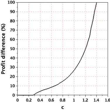
As shown in Appendix A.3, when the conditions of Lemma2 hold, x= 1 is theunique

equilibrium if and only if γ satisfies

γ < c+ 2δh+ 2 p

(c/2 +δh)(δr+δh). (3.21)

This then ensures that adoption increases monotonically until reaching full adoption. The

condition of Eq. (3.21) can be combined with Lemma2 to obtain the equivalent of

Propo-sition 1for the hybrid pricing policy.

Proposition 2. Under the hybrid pricing of Eq. (3.19), full adoption, x=1, is the unique

equilibrium if and only if

• When γ < c: δh >0 and δr >−δh

• When γ ≥c: δh >0 and δr >−δh and

δh >

γ2 4(γ+δr−c/2)

−c/2. (3.22)

Proof. As a result of the two conditions δh >0 and δr>−δh and because c≥0 it follows

that 2δh + 2 p

(c/2 +δh)(δr+δh) in Eq. (3.21) is always positive. Therefore Eq. (3.21)

always holds ifγ < c, without further constraints on the values of δh and δr.

On the other hand, when γ ≥ c, δh and/or δr need to be large enough to ensure that

Eq. (3.21) is satisfied. Specifically, algebraic manipulation of Eq. (3.21) in this case yields

Eq. (3.22).

Proposition 2 states that when x = 1 is an equilibrium under hybrid pricing, it can

coexist with other equilibria when the value of home connectivity utility is high enough,

i.e., γ ≥c and the condition of Eq. (3.22) is not satisfied. Focusing on cases when x = 1

maximizes total welfare,e.g.,eis low enough, this means that it is possible for the provider

to set pricesph and pr (and consequentlyδh and δr) for which full adoption is feasible,i.e.,

(42)

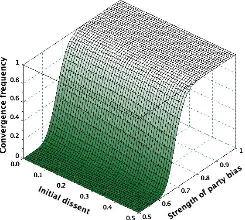
Figure 3.5: Final adoption level for the hybrid pricing policy, and identification of the boundaries demarcating the regions associated with the conditions of Proposition 2. The straight line corresponds to γ = c = 0.8, and the curved line captures the condition of Eq. (3.22). The system’s parameters arec= 0.8, δr = 0, withγ and δh values varying.

occurs when the provider’s choice of prices allows the emergence of a second equilibrium

e

x <1, where adoption stops upon reaching it.

As Proposition 2 indicates though, it is possible to avoid such outcomes by properly

selecting prices (parameters δh and δr) to comply with Eq. (3.22). This is illustrated in

Fig. 3.5, which plots the system’s final adoption as γ and δh vary for the case c = 0.8

(initial adoption is set to x = 0, and for simplicity we assume δr = 0 and focus on the

impact of varying δh). The figure confirms (straight boundary line at γ =c = 0.8 in the

figure) that when γ < c= 0.8, any value of δh > 0 results in full adoption. It also shows

that when γ ≥c= 0.8, the system only converges to full adoption whenδh further satisfies

the condition of Eq. (3.22) (corresponding to δh values that lie to the right of the curved

boundary line in the figure).

The conditions of Proposition 2 are clearly specific to the assumptions on which the

model is predicated. However, we will see in Section 3.9 that the very same behavior

arises under more general settings; specifically, a second, sub-optimal equilibrium (x <_e 1)

can arise whenever the value of home connectivity exceeds a certain threshold, and in the

(43)

overcoming this issue can again be accomplished by adjusting prices, albeit to different

values than those of Proposition2.

We note that the aspect of adjusting (lowering) prices to ensure full adoption begs the

question of what would motivate the provider to do so. We explore this issue next in the

broader context of the hybrid pricing policy’s ability to distribute welfare between users

and the provider. We first explore the pricing policy’s ability to support arbitrary welfare

distribution at full adoption, including maximizing the provider’s profit, and then focus on

the extent to which the conditions of Proposition2constrain this ability, and what options

are available to overcome those limitations.

3.6.3 Welfare Distribution

As before, we focus on scenarios for which total welfare is maximized at full adoption,i.e.,

combinations that, as illustrated in Fig. 3.1, correspond to a low enough cost erelative to

the other system’s parameters γ, c, and r. We explore first whether, once at full adoption

(and maximum total welfare), the hybrid pricing policy allows an arbitrary distribution of

welfare (as the usage-based policy did), from maximum user welfare to maximum provider

profit.

Lemma2identifies the constraints that pricing must satisfy to ensure that full adoption

is an equilibrium, i.e.,δh>0 andδr>−δh. Combining Eq. (3.20) and Eq. (3.7) gives the

following expression for the users’ welfareWU([0,1]) at full adoption

WU([0,1]) =δh+ δr

2 , (3.23)

with according to Eq. (3.13) and Eq. (3.11), the provider’s profit given by

WP([0,1]) =

γ+r−c

2 −e−

δh+

δr 2

. (3.24)

(44)

according to Eq. (3.24) implies

δh+ δr

2 =

γ+r−c

2 −e.

This can be readily accomplished by choosing values ofδh andδrthat also satisfy Lemma2,

e.g., δh = >0, and δr=γ+r−c−2e−2 >−, whereis arbitrarily small. Conversely,

maximizing the provider’s profit calls for setting prices that extract (nearly) all the value

users realize from the system, i.e., set both δh and δr equal to arbitrarily small positive

values (this again satisfies the conditions of Lemma2, namely,δh>0 andδr >−δh).

Intermediate distributions of welfare are also feasible simply by adjusting the values of

δh and δr. Consider for example a scenario where a regulator wants all users to see the

same utility valueα >0. From Eq. (3.20) the utility of a user with roaming parameter θis

given by

U([0,1], θ) =δh+θδr=α .

Eliminating the dependency onθto ensure that all users see the same utility requiresδr= 0,

which then implies δh =α >0 that again satisfies the conditions of Lemma 2. Hence, we

see that once at full adoption (and assuming full adoption maximizes welfare), the hybrid

pricing policy, like the usage-based policy, is capable of achieving any arbitrary distribution

of welfare between users and the provider. However as made explicit in Proposition 2,

reachingfull adoption can, as reflected in Eq. (3.22), impose additional conditions on pricing,

which may preclude some welfare distribution configurations. In particular, maximizing the

provider’s profit, which as just discussed calls for setting bothδh andδr to arbitrarily small

positive values, readily conflicts with the conditions of Eq. (3.22).

A possible approach suggested by the discussion of Section 3.6.2, is for the provider to

offer anintroductory pricing that satisfies the conditions of Proposition2; thereby enabling

full adoption to be reached. The motivation for the provider to do so is that once full (or

nearly full12) adoption has been reached, it can then switch to a pricing scheme that allows

12

(45)

it to extract a higher profit.

In the next section, we introduce a third family of pricing policies that seeks to eliminate

all dependency on monitoring a user’s usage; therefore simplifying implementation and

possibly facilitating user acceptance.

3.7 Fixed Price Policy

This section considers a pricing policy based on a fixed price that covers both home and

roaming connectivity.

As mentioned earlier, the use of a fixed price is not uncommon for home connectivity,

but it is arguably less so for wireless roaming access which is the other component of the

service we consider. Nevertheless, a number of wireless carriers do offer fixed-price wireless

services [89]. Hence it is of interest to investigate the impact such a pricing policy might

have on their ability to maximize profit and on the welfare the system realizes.

Pricing is independent of usage and based on a single parameter p,

p(Θ, θ) =p, ∀Θ, θ. (3.25)

We investigate if and how p can be set to realize maximum welfare and flexibility in

dis-tributing it across stakeholders. As per the discussion of Section3.4, the former (typically)

calls for selectingp so as to ensure full adoption,i.e., x= 1.

3.7.2 Maximum Service Adoption

Given Eq. (3.5) and the price structure of Eq. (3.25), the utility of user θ is

Decision Making in Networked Systems

University of Pennsylvania

ScholarlyCommons

Publicly Accessible Penn Dissertations

1-1-2015

Decision Making in Networked Systems

Mohammad Hadi Afrasiabi

Follow this and additional works at:

http://repository.upenn.edu/edissertations

Part of the

Engineering Commons

Recommended Citation

Decision Making in Networked Systems

Decision Making in Networked Systems

Contents

Chapter 1

Introduction

1.1

Adoption of service in user-provided connectivity

1.2

Opinion formation in biased networks

Chapter 2

Related works

2.1

Adoption of products and services

2.2

Formation and spread of opinions

Chapter 3

User-Provided Connectivity

3.1

Introduction

3.2

Model Formulation

3.3

Total Welfare

3.4

Role of Pricing

3.5

Usage-based Pricing Policy

3.6

Hybrid Usage-based Pricing Policy

3.7

Fixed Price Policy