Measurement of Error in 3D Polygonal Model Using MAYA API

(1)

Measurement of Error in 3D Polygonal

Model Using MAYA API

R.Rama Kishore, Prof. Yogesh Singh, Prof. B.V.R.Reddy

Abstract

Generally applications in computer graphics use very high detailed models. These models are too complex for the limited hardware capacity and take much time to render and to transmit. Related fields can benefit from simplification of complex polygonal models. This introduces errors in the models during the process of simplification. It is required to measure the error in the model during simplification to judge the quality of the 3D model. This paper proposes a fast and easy method to estimate the error in 3D models as a valuable tool for managing data complexity. This algorithm is implemented on 4 different sets of models. Each set contains models at different number of polygon levels. Experiments are repeated to measure error on them at each level. In order to gain in both memory and speed, VC++ API is developed and created a MLL (Maya link library) to load as a plug-in in Maya.

Index Terms: Error metric, MAYAAPI, Plug–in.

I. Introduction

Computer graphics applications require complex 3 dimensional models to maintain a convincing level of realism. Large quantities of complex 3 dimensional models having large set of polygons are available. More number of polygons are required to get efficient realism in the model. But large amount of polygons i.e. larger details are not required for the applications where attributes like hardware capacity, processing time, transmission speed and rendering time are of prime concern [6]. Hence there is a need to simplify the 3D model. Simplification of a 3 D model means to reduce the number of polygons making that model. Simplification begins with a geometric description of an object and produces a new description that is similar in appearance to the original with few geometric primitives. But if we reduce the polygons the quality of model gets affected as there is a trade-off between quality and those 4 factors (processing time, hardware capacity, transmission time, rendering time). In 3D models many of the errors are introduced during the process of polygonal simplification. Sometimes we need to apply some method to judge the quality of the new output with respect to the previous one [7].

Hence the focus of this work is to generate fast and easy method which measures the error in the model while maintaining the quality (less compromise in quality).

The error measurement is a measure of differences between two polygonal models. Small error between two models means they are very much similar to each other. An error measurement is usually required to define as the geometric distance between an original and a simplified model. Some error measurement combine other attributes – color, normal, and texture values apart from the geometric details to ensure or differentiate the appearance during the manipulation of 3D models.

Because of the dependency of human vision on intuition and limitations of human persistence of vision a mathematical model is always preferred to be used as an error metric Human metric system is not very reliable and fails after certain limit. Thus a mathematical method is required to evaluate the error between models with the same accuracy and efficiency all the time [8, 10]. A consistent and quantitative method is required to get a consistent and accurate result again and again. Use of a good measuring error will always improve the final quality of the simplified model.

(2)

The primary aim of measuring error is to compare the given model that is as similar as possible to the original model. In order to assess the quality of the model, some means of quantifying the notion of similarity is required in terms of geometry and as well as appearance. This paper uses geometry error to compare the models. In this work, a method which measures the average squared distance between the model with complex data ie original and simplified data ie simplified is used. So the error that is Ei will be defined as [16]:









_

















 Xn V Xi V

i i

n

i

d

V

M

d

V

Mn

X

E

1

2

,

2

,

Where

X

i

,

X

n_{are sets of points sampled on the models}_Mn

(original model) and Mi (simplified) respectively. The distance d(v, M) is the minimum distance from v to the

closest face of M. Using the above equation, the error will be calculated by comparing the quality the original, simplified models.

3.1 Few important classes used in the API programming 3.1.1 MFnMesh

MFnMesh contains several methods for retrieving mesh specific data and modifying a mesh. one could use an iterator to find a particular component and use MFnMesh to perform an operation on that component. This function set provides access to polygonal meshes.Objects of type MFn::kMesh, MFn::kMeshData, and MFn::kMeshGeom are supported.

3.1..2 MitDag

It can traverse the DAG (Directed Acyclic Graph) either depth first or breadth first, visiting each node. MItDag provides the capability to not only traverse the DAG and to retrieve specific nodes for subsequent query and edit using compatible Function Sets.

3.1.3 MDagPath

Provides methods for obtaining one or all Paths to a specified DAG Node, determining if a Path

is valid and if two Paths are equivalent. DAG Paths may be used as parameters to some methods in the DAG Node Function Set (MFnDagNode). It is often useful to combine DAG Paths into DAG Path arrays (MDagPathArray). DAG Path Class is used to obtain and query Paths to DAG Nodes. A DAG path is a path from the world node to a particular object in the DAG.

Algorithms being used

1. Extracting all polygonal model data like vertices, edges and faces from the original model(M1) and store in

a file1

2. Extracting all polygonal model data like vertices, edges and faces from the simplified model(M2) and store in a file2

3. Distance from point on M1 to the all faces of M2 is computed.

4. Minimum of these distances is squared and added to sum1 5. Step3 and 4 are repeated on all the points of model M1

6. Steps 3,4 and 5 are done by changing M1 to M2 and M2 to M1 to calculate the sum2

(3)

IV. Experimentation

In this work, VC++ API is developed and created a MLL (Maya link library) to load as a plug-in through Maya plug-in manager. Plug-in is called through a MEL command when ever evaluation of the model is required. The error of the model is displayed in the out put screen in terms of scaled unit distance of MAYA.

Four different sets of models have been considered for in this work. These models sets are:

1. Rubber Duck 2. Space Ship 3. Face 4. Bottle

(1) Rubber Duck Model:

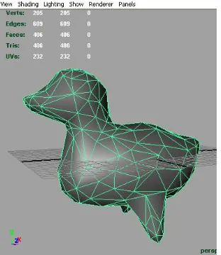
Duck model was taken at 9 different levels and error was measured through plug in and the details are as follows.

Fig 4.1.1 Duck model with no of polygons:456

(4)

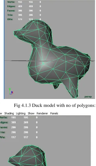
Fig 4.1.3 Duck model with no of polygons: 306

Fig 4.1.4 Duck model with no of polygons:206

(5)

No of faces Error Ei 456 0.000096864 406 0.000064205 356 0.000155429 306 0.000362701 256 0.000673325 206 0.00195359 156 0.0127583 106 0.015121 56 0.0481964

Table 4.1 No of faces versus Error (Ei) of Duck model

Comparison between no of faces and Error Ei(Rubber Duck)

0.00001 0.0001 0.001 0.01 0.1 1 45 6 40 6 35 6 30 6 25 6 20 6 15 6 10 6 56

No of Faces

Er

ro

r Ei

(2) Space Ship

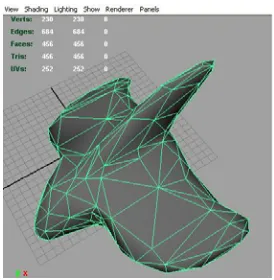
Space ship model was taken at 10 different levels and error was measured through plug in and the details are as follows.

(6)

Fig 4.2.2 Space ship model with no of polygons: 456

(7)

No of faces Error Ei

956 0.000270105 856 0.000894437 756 0.00172094 656 0.00305895 556 0.00487016 456 0.00848853 356 0.0162855 256 0.0274323 156 0.11192 56 1.523144

Table 4.2 No of faces versus Error (Ei) of Space ship model

Comparision between no of faces and Error Ei(Space Ship)

0.0001 0.001 0.01 0.1 1 10 95 6 85 6 75 6 65 6 55 6 45 6 35 6 25 6 15 6 ₅₆

No of Faces

Er

ro

r Ei

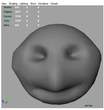
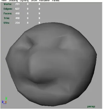
(3) Face Model:

(8)

Fig 4.3.1 Face model with no of polygons: 1218

(9)

1218 0.0000337189 1118 0.000106353 1018 0.000234891 918 0.000413079 818 0.000786858 718 0.00129743 618 0.00272118 518 0.00446441 418 0.0077195 318 0.0181178 218 0.0388773 118 0.0880551

(10)

0.00001

No of Faces

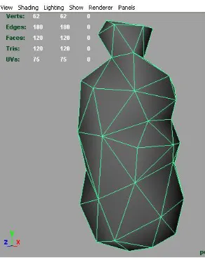
(4)Bottle model:

Bottle model was taken at 12 different levels and error was measured through plug in and the details are as follows

Fig 4.4.1Model with no of polygons: 1120

(11)

Fig 4.4.3 Model with no of polygons 320

Fig 4.4.4 Model with no of polygons 120

(12)

No of faces

V. Conclusions

An error measuring approach is proposed in this work that is capable of measuring error of the polygonal models. This is implemented through API programming and effectively used as a plug-in in MAYA. This can track the approximate error of the model while it is being simplified. Error measurement is done at different levels of model in each set. Four different sets are taken for the same. The results are convincing as the trend is found to be like error is inversely proportional to the no of polygons. Error is increasing as the numbers of polygons are decreasing. This approach of measuring error of 3D model is useful to determine the error of any surface to decide the optimum surface levels with greater speed and flexibility.

This method can be made utilized to optimize the working time on 3D model in respect to rendering time, transmission of 3D models over networks and 3D data compression.

Models can be set at complexity of polygonal data that is reasonable to the user as per availability of the hardware capabilities.

VI. Future Direction

Quality optimization: This error measuring approach can be combined with some error metric techniques to simplify the surfaces for optimizing the quality.

Improved Error Analysis: The error Ei that has been taken as to evaluate the simplified model in terms of surface geometry. Similar approaches can be used to evaluate the error Ei considering similarity of appearance, color and texture values etc.,

The same may be repeated on existing tools like Metro, poly Meco and comparative analysis can be made. References

[1] Herv´e Delingette. Simplex meshes: a general representation for 3D shape reconstruction. Technical report, INRIA, Sophia Antipolis, France, Mar. 1994. No.2214,

[2] Michael Lounsbery. Multiresolution Analysis for Surfaces of Arbitrary Topological Type. PhD thesis, Dept. of Computer Science and Engineering, U. of Washington, 1994.

[3] Matthias Eck, Tony DeRose, Tom Duchamp, Hugues Hoppe, Michael Lounsbery, and Werner Stuetzle. Multiresolution analysis of arbitrary meshes. In SIGGRAPH ’95 Proc., pages 173–182. ACM, Aug. 1995.

[4] Yun-Sang Kim, Sebastien Valette, Ho-You Jug, and Remy Prost. Local Wavelets Decomposition for 3-D Surfaces. In 1999 [5] Jihad El-Sana and Amitabh Varshney. Feneralized View- Dependent Simplification ,Volume 18,1999, EUROGRAPHICS. [6] Paul Hinker and Charles Hansen. Geometric optimization. In Proc. Visualization ’93, pages 189–195, San Jose, CA, October 1993. [7] Alan D. Kalvin and Russell H. Taylor. Superfaces: polygonal mesh simplification with bounded error. IEEE Computer Graphics and Appl.,

16(3), May 1996.

[8] Amitabh Varshney. Hierarchical Geometric Approximations. PhD thesis, Dept. of CS, U. of North Carolina, Chapel Hill, 1994. TR-050. [9] Marc Soucy and Denis Laurendeau. Multiresolution surface modeling based on hierarchical triangulation. Computer Vision and Image

Understanding, 63(1):1–14,1996.

[10] Reinhard Klein, Gunther Liebich, and W. Straßer. Mesh reduction with error control. In Proceedings of Visualization ’96, pages 311–318, October 1996.

[11] Martin Franc, Vaclav Skala. Parallel Triangular Mesh Decimation With out Sorting. In 2001

[12] Andr´e Gu´eziec. Surface simplification with variable tolerance. In Second Annual Intl. Symp. on Medical Robotics and Computer Assisted Surgery (MRCAS ’95), pages 132–139, November 1995.

[13] Alexis Gourdon. Simplification of irregular surface meshes in 3D medical images. In Computer Vision, Virtual Reality, and Robotics in Medicine (CVRMed ’95), pages 413–419, Apr. 1995.

(13)

[15] Hugues Hoppe. Progressive meshes. In SIGGRAPH ’96 Proc., pages 99–108, Aug. 1996.

[16] Garland, Michael and Paul Heckbert, “Surface Simplification using Quadric Error Metrics ”, Proceedings of SIGGRAPH 97. pp. 209-216. [17] Klein, Reinhard, Gunther Liebich, and Wolfgang Straßer, “Mesh Reduction with Error Control”, Proceedings of IEEE Visualization '96.

[18] L.H. You,Javier Romero Rodriguez,Jian J.Ahang.,”Manupulation of Elastically Deformable Surfaces through Maya Plug-in”, Proceedings of the Geometric Modelling and imaging- New Trends,IEEE2006.

[19] A.M.Day,D.B. Arnold, S.Havemann, D.W. Fellner, “Combining Polygonal and subdivision Surface approaches to modeling and rendering of urban environments”,Computers &Graphics 28(2004) 497-507. ELSEVIER

[20] Muhammad Usman Keerio, Abdul Fattah Chandio, Attaullah Khawaja and Ali Raza Jafri , “ Virtual Scene for Telerobotic Operation”,

International Conference on emerging Trends IEEE2006.

[21] Yacine Amara, Mario Gutiérrez, Frédéric Vexo and Daniel Thalmann, “A MAYA Exporting Plug-in for MPEG-4 FBA Human Characters”, infoscience.epfl.ch/record/100258/files/Amara_and_al_Richmedia_03.pdf