Co-evolving the Operators of Variation
Bruce Edmonds,
Centre for Policy Modelling,
Manchester Metropolitan University,
Aytoun Building, Aytoun Street, Manchester, M1 3GH, UK. Tel: +44 161 247 6479 Fax: +44 161 247 6802
E-mail:[email protected] URL:http://www.fmb.mmu.ac.uk/~bruce
Abstract
The standard Genetic Programming approach is augmented by co-evolving the genetic operators. T o do this the operators are coded as trees of indefinite length. In order for this technique to work, the language that the operators are defined in must be such that it preserves the variation in the base population. This technique can varied by adding further populations of operators and changing which populations act as operators for others, including itself, thus to provide a framework for a whole set of augmented GP techniques. The technique is tested on the parity problem. The pros and cons of the technique are discussed.
Keywords
1. Introduction
Evolutionary algorithms are relatively robust over many problem domains. It is for this reason that they are often chosen for use where there is little domain knowledge. However for particular problem domains their performance can often be improved by tuning the parameters of the algorithm. The most studied example of this is the ideal mix of crossover and mutation in genetic algorithms. One possible compromise in this regard is to let such parameters be adjusted (or even evolve) along with the population of solutions so that the general performance can be improved without losing the generality of the algorithm1. The most frequently quoted is [4], which investigates the incremental tuning of parameters depending on the success of the operators in initially converged populations.
Such techniques have also been applied in genetic programming (GP)2. This usually involved the storing of extra information to guide the algorithm, for example in [2] extra genetic material is introduced to record a weight ef fecting where the tree-crossover operator will act. As [1] says, “There is not reason to believe that having only one level of adaption in an evolutionary computation
is optimal” (page 161).
In genetic programming the genetic operators are usually fixed by the programmer . Typically these are a variety of crossover and propagation, but can also include others, for example mutation. A variety of alternative operators have been invented and investigated (e.g. [2]). It is usually found that, at least for some problems these preform better than the ‘classic’ mix3 of mostly tree-crossover and some propagation (e.g. [3]).
Meta-Genetic Programming (MGP) encodes these operators as trees. These “act” on other tree structures to produce the next generation. This representation allows the simultaneous evolution of the operators along with the population of solutions. In this technique what is co-evolved along with the base population is not a fixed set of parameters or extra genetic material associated with each gene, by operators who are themselves encoded as variable length representations – so their form as well as their preponderance can be evolved..
This technique introduces extra computational cost, which must be weighed against any advantage gained. Also the technique turns out to be very sensitive to biases in the syntax from which the operators are generated, it is thus much less robust.
Iterating this technique can involve populations of operators acting on populations of operators acting on populations etc., and even populations acting on themselves. This allows a range of techniques to be considered within a common framework - even allowing the introduction of deductive operators such as Modus Ponens to be included.
In section 2., I describe the basic technique in more detail. In section 5., I describe the use of possible elaborations of MGP to provide a coherent framework for the analysis of a wide range of such structures. I test a few configurations of MGP on the parity problem at dif ferent levels of difficulty in section 4., followed by a general discussion (section 7.). I finish with a small sample of the further work that needs to be done about this technique in section 8..
2. The Basic Technique
Instead of being hard-coded, the operators are represented as tree structures. For simplicity this is an untyped tree structure in the manner of Koza [8]. Two randomly chosen trees along with randomly chosen nodes from those trees are passed to be operated on by the operator tree. The terminals refer
to one or other of these trees at the respective node. The structure of the operator tree represents transformations of this (tree, node) pair until the root node produces the resulting gene for the next operator.
Thus there could be the following terminals:
rand1 - return the first, randomly chosen gene plus random node;
rand2 - return the second, randomly chosen gene plus random node;
bott1 - return the first, randomly chosen gene plus the root node;
bott2 - return the second, randomly chosen gene plus the root node. and the following branching nodes:
top - cut the passed tree at the passed node and return it with the root node;
up1 - pass the tree as it is but choose the node immediately up the first branch;
up2 - pass the tree as it is but choose the node immediately up the second branch;
down - pass the tree as it is but choose the node immediately down;
down1 - identical todown (so that the operators will not have an inherent bias up or down);
subs - pass down a new tree which is made by substituting the subtree at the node of first argument with for the subtree in the second at the second’s indicated node.
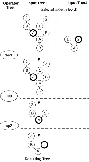
For example if the operator,[up2 [top [rand1]]] were passed the following input pair of (tree, node) pairs to act upon, ([B [A [A [B [2]] [1]] [3]]],[1 1]), ([A [1] [2]],[2]) it would return the pair ([A [B [2]],[2])4 – this process is illustrated below in figure 1.
Figure 1: An example action of an operator on a pair of trees with selected nodes up2
top rand1
B A
A B
B 2
1 3
A
1 2
B A
A B
B 2
1 3
A B 2
1
A B 2
1 Operator
Tree
Input Tree1
(selected nodes inbold)
Input Tree1
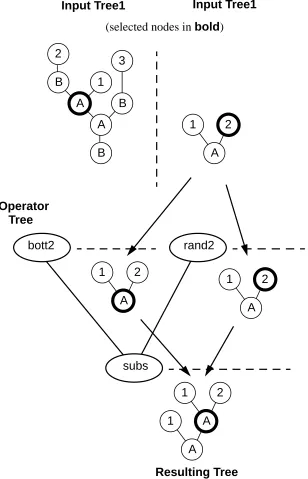
A second example is if the operator , [subs [bott2] [rand2]] were passed the same inputs it would return ([A [1] [A [1] [2]]],[2]) – as illustrated in figure 2.
Figure 2: A second example of an operator acting on a pair of trees with selected nodes
Thus a cut&graft operator (one half of a traditional GP crossover) could be represented like this (figure 3).
Figure 3: A cut and graft operator encoded as a tree B
A
A B
B 2
1 3
A
1 2
Operator Tree
Input Tree1
(selected nodes inbold)
Input Tree1
Resulting Tree
bott2 rand2
subs
A
1 2
A
1 2
A 1 A
1 2
subs
This takes the first random gene, cuts off the top at the randomly chosen position and then substitutes this for the subtree at the randomly chosen position of the second chosen gene. The single leafrand1
would represent propagation.
The population of operators is treated just like any other genetic population, being itself operated on by another population of operators. This sequence must eventually stop with a fixed non-evolving population of operators or a population that acts upon itself.
The base population and operator population(s) will have different fitness functions - the basic one determined by the problem at hand and the operator ’s function by some measure of success in increasing the fitness of the population they operate on.
3. Short-term Operator Success and Population Variation
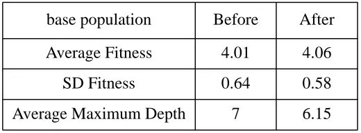
Initial trials of the technique failed. It was discovered that this was due to the fact that the variation in the base population was too quickly destroyed. T o show this an experiment was run where a population of 200 randomly generated operators of depth 5 in the language described above, acted on a population of 10,000 base genes of depth 7 using nodes AND, OR and NOT and terminals
input-1,...,input-3. The operators were applied to 50 pairs of input genes each, which were chosen with a probability proportional to their initial fitness (as in standard GP). The fitness of the base population was evaluated on the even parity 3 problem before and after the application of the operators. The effect of the operators was evaluated by the average change in fitness of the operand genes before and after, where binary operators were evaluated by comparing the average of the input genes compared to the result.
Not surprisingly, there was only a slight improvement in the population fitness (and marginally worse than what would have been achieved by fitness proportionate selection alone), but the variation of fitnesses and the average maximum depth of base genes significantly diminished, indicating a destruction of the variation in the base population. The overall statistics are shown in table 1, below.
Table 1: Overall Statistics of Experiment
Firstly, the operators which were ef fectively binary increased the fitness of the population by significantly less than those that were only unary . It was not that the unary operators were particularly good at increasing fitness, just that, on average, the binary operators were worse than average - this is illustrated in figure 4 (operators that were strictly equivalent to straight propagation are excluded to aid the scaling - there were 59 of these, all unary of course).
base population Before After
Average Fitness 4.01 4.06
SD Fitness 0.64 0.58
Figure 4: Comparison of Distributions of Fitness Change Caused by Operators
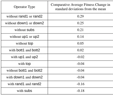
I analysed the operators into those with and without certain nodes and terminals, the results are shown in table 2, in terms of standard deviations of fitness changes from the mean fitness change.
Table 2: Table of comparative effect in terms of average fitness change by operator type
The presence (or absence) of substitution, random node choice (as opposed to starting at the root) and the lack of movement up or down, were most significant in af fecting fitness change. This, however may be problem specific. What is not apparent from the above is that operators which corresponded in effect to a standard half of a crossover operator , did less well than the average in improving the fitness of the base population (on average they decreased the fitnesses by a factor of
Operator Type Comparative Average Fitness Change in standard deviations from the mean
withoutrand1 or rand2 0.29
withoutdown1or down2 0.25
withoutsubs 0.21
withoutup1 or up2 0.14
withouttop 0.05
withbott1andbott2 0.02
withup1and up2 -0.02
withtop -0.04
withoutbott1and bott2 -0.04
withdown1 and down2 -0.04
withrand1 and rand2 -0.16
withsubs -0.18
0.93-0.95 0.95-0.97 0.97-0.99 0.99-1.01 1.01-1.03 1.03-1.05 1.05-1.07 0
5 10 15 20 25 30 35
Intervals of Average Fitness Increase due to Operators
0.98), but were good at preserving variety. This indicates that short-term average increase in fitness may be less important than the occasional discovery of sharply better solutions while preserving variety.
What is more important is the ef fect on the population variation. This is guessed at via the variation in fitnesses of used and resulting genes from the ground population. This is shown in table 3.
Table 3: Effect on variation of fitness of types of operators
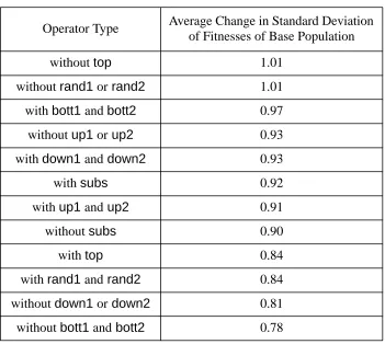
Here we can see the significant effect of the presence or otherwise of top,rand andbott type nodes in an operator. It would seem that omitting eithertop orrand1 &rand2 will have the effect of preserving the variation in the population. I chose to omit bothtop andrand1 &rand2 as the above table suggest that the ef fect of this might be to maximise the increase in fitness as but without the overall bias of the operator language being towards destruction of variety (as it indeed turned out). As we shall see this did have the effect of preserving the base population’s variety while allowing the operator population to evolve.
4. Preliminary Test Results
The main practical questions to be resolved with respect to MGP are whether using this technique leads to improved results and whether such improvements are worth the additional computational cost. To do this a straight comparison of the number of evaluations of the base population is unfair as when using MGP one has to also evaluate the operator population as well. Thus if one has a base population of 600 in both cases and an operator population of 200 in the second case execution time is increased by a factor of about 1.33. This is a bit rough and ready but seems to give a reasonably fair comparison reflecting computational times in practice.
Operator Type Average Change in Standard Deviation of Fitnesses of Base Population
withouttop 1.01
withoutrand1or rand2 1.01
withbott1andbott2 0.97
withoutup1or up2 0.93
withdown1and down2 0.93
withsubs 0.92
withup1and up2 0.91
withoutsubs 0.90
withtop 0.84
withrand1and rand2 0.84
withoutdown1or down2 0.81
I chose a problem that was deliberately straight-forward, but not too easy for simple GP
algorithms: the 4-parity problem allowing nodes of AND, OR and NOT only , nodes for the four possible inputs, using base populations of 600. The fitness function was the number of correct cases the gene made (out of the total of 16), with a slight penalty for depth which can never be greater than one. The initial population was randomly generated with an even depth of 7.
The MGP algorithm had in addition a population of 200 operators using nodes up1, up2,
down,down1 andsubs with terminals ofbott1 andbott2 (as described in section 2. above). This is turn was operated on by a population of 9 cut-and-graft operators (as illustrated in figure 3) and one simple propagation operator, all with fixed equal weights (as illustrated in figure 13). This population was also initially randomly generated with an even depth of 6. The fitness function for this population was found to be critical to the success of MGP . The basic fitness was the average proportionate change effected in the fitnesses of the base genes it operated upon. There were several (necessary) elaborations on this basic function: the fitnesses were smoothed by a running average over the last 3 generations; new genes were accorded a fitness of 1; and genes that had no ef fect on the fitness of genes (i.e. they were essentially propagation operators) were heavily discounted. (otherwise these came to quickly dominate the population as most ‘active’ operators had a fitness of less than one).
The MGP version had, in addition, two further modifications, found necessary to make it run successfully. Firstly, there was a depth limitation of 15 imposed, as the MGP algorithm is susceptible to hyper-inflation (this is potentially far worse than in a GP algorithm as an operator with multiple
subs operations can be evolved). Secondly, in the MGP algorithm fitness dif ferentials were vastly magnified by a ranking mechanism, this was necessary in the operator population because of the small differences in their fitnesses but was also because MGP introduces a higher level of variation into the base population so a stronger selection force is needed (in the GP algorithm a shifted fitness proportionate system was used as the GP performed worse under a ranking system).
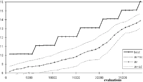
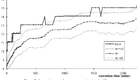
Both algorithms were implemented in the high-level declarative language SDML5, with some time critical sections implemented in VisualWorks/Smalltalk. The execution times are both for the same Sun 5 Sparcstation. In figure 5 the average fitness and the fitness of the best individual is shown vs. execution time; the dotted lines are plus and minus one standard deviation of the population fitnesses and the crosses indicate when the generations occurred.
Figure 5: Best and average fitness vs. execution time for MGP run
Figure 6: Best and average fitness vs. number of evaluations for MGP run
Thus in the best run of the MGP algorithm it found a perfect solution after 36 generations (28,800 evaluations) and 1050 minutes of execution time. Compare this to the results in figure 7 for the best GP run obtained. This only found the perfect solution after 93 generations (55,800
execution time (mins)
fitness
evaluations
evaluations) and 2380 minutes of execution time. The same number of runs were made of each (6). Although the best run in each case is shown, these results are typical.
Figure 7: Best and average fitness vs. execution time for GP run
Figure 8: Best and average fitness vs. number of evaluations for GP run
There are several things to note. Firstly, that in the MGP algorithm the learning is much smoother than in the GP algorithm - this may indicate that the MGP algorithm is acting as a more greedy but less robust search of the space of solutions. Secondly, that the MGP algorithm slows
down a lot more quickly than the GP algorithm - this is due to the rapid inflation as the MGP algorithm learns to “grow” the base population to a greater depth. Such inflation is almost inevitable due to the distribution of solutions of dif ferent depths, as shown in figure 9 - there are just many
execution time (mins)
fitness
evaluations
more better solutions accessible using a greater depth of candidate gene (this is further explored in [9]). This may be another advantage of GP, as it inflates the population much more slowly. Thirdly, that while both techniques maintain a good level of variation in their base populations, the GP algorithm not only has a higher level of variation, but also increases the level of variation as it progresses (although it is possible that this is due to the fitness proportionate system of selection compared to the ranking system used in the MGP algorithm). Again this might indicate the greater robustness of standard GP over MGP.
Figure 9: Distribution of 50,000 randomly sampled propositional expressions of different depths in
four variables using AND, OR and NOT compared to the parity function
What may not be immediately obvious from the graphs above is the difference in the shapes of the curves. In figure 10 we compare the curves of best and average fitnesses on the same axis of execution time. Here we see that, although the GP algorithm did better at the start, both in terms of best and average fitness, the MGP algorithm did not seem to suf fer the characteristic flattening out
Number of Wrong Consequents Maximum Depth of
Logical Expression Log of
that occurs in GP algorithms (at least, not anywhere to the same extent). It is perhaps this that indicates most clearly the potential of the MGP approach.
Figure 10: Comparing the MGP and GP runs
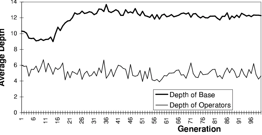
However, as mentioned above the technique is susceptible to hyper -inflation as well as being somewhat brittle to other modifications. For example, if a ceiling is placed on the maximum depth of candidate solutions this can destroy the ef fectiveness of the MGP algorithm. In figure 11 and figure 12, I show the results of a run where a depth limit of 14 is imposed (for the same even parity 4 problem). It is evident that as soon as the ceiling is reached (after about 40 generation) the algorithm ceases to be effective.
Figure 11: Average Depth in MGP run with a Depth Ceiling of 14
execution time (mins)
Figure 12: Average Depth in MGP run with a Depth Ceiling of 14
5. MGP as a framework for a set of techniques
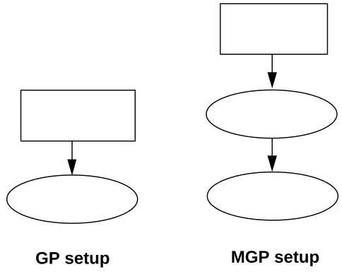
The relation of “Population A acting as operators on population B” can be represented diagrammatically by an arrow. In figure 13, I illustrate traditional GP and basic MGP setups, with evolving population represented by ellipses and fixed populations by rectangles.
Figure 13: GP and MGP setups
There is no a priori reason why many different setups should not be investigated. For example figure 14 shows a simple enhancement of GP where just the proportions of the operators is changed, implementing a similar technique as invented by for GAs, and figure 15 illustrates the possibility of combining a fixed and evolving population of operators.
base population crossover propagation
base population operator population
crossover propagation
Figure 14: GP with the proportion of operators evolving
Figure 15: A setup with a mixture of fixed and evolving operators
Finally there is no reason why populations of operators should not operate recursively. One can even imagine situations in which the interpretation (i.e. fitness) of the base population and operator population was done consistently enough such that you only had one population acting on itself in a self-organising loop, as in figure 16. In this case care would need to be taken in the allocation of fitness values, maybe by some mechanism as the bucket-brigade algorithm [6] or similar. Such a structure may allow the implicit decision of the best structure and allow for previously unimaginable hybrid operator-base genes6. It does seem unlikely, however, that the same population of operators would be optimal for evolving the operators as the base population, due to their different functions.
6. In this way it is similar to a suggestion by Stuart Kauffman [7] for a computational model of enzymes that act upon each other.
base population operator population propagation
crossover propagation
base population
operator population
Figure 16: A recursively evolving MGP setup
Further, if the language of the operators described above could be extended with the addition of nodes like “ if-then-else”, “equal”, “and” and “root-is-implies” nodes, then operators like Modus Ponens (the logical rule that says from and you can infer ) could be encoded (see figure 17). This would mean that such an operator would produce child genes which were the logical inferences of those in previous generations. Such an operator would produces deductions on the genes. In a similar way one could allow for a techniques which allow dif ferent mixes of inferential and evolutionary learning techniques.
Figure 17: A Modus Ponens operator
In this way the dif ferences between approaches become less marked, allowing a range of mixed learning approaches to tried. It also provides a rudimentary framework for them to be compared.
6. Related Research
Most of the work done in investigating self-adapting evolutionary algorithms has fallen into one of three camps: those which add extra genetic material to the genome (this includes ADF and ADM techniques as well as those such as [2]); those that build up a central library of modules and hence change the language of gene expression; and those which adapt a fixed set of parameters. The work descried here does something different in that the operators are adapted in form as well as propensity to be used – in other words I have moved from co-evolving a fixed block of material to a variable length representation of the evolutionary set-up.
This is not the first time that co-evolving the genetic operators has been proposed. T eller [14] suggests the co-evolution of programs to perform operations of variation on other programs. In that
base population operator population
A B A B
if then else up1
bott1
bott1 bott2
up2
equal
bott2 top
and bott1
evolved operators is that there is no obvious operator that would correspond to a GP “crossover” operator. MGP is conceptually much simpler and hence may enable more opportunities for meaningful analysis. Furthermore because it is uses a straightforward GP algorithm on the operator population, some of the analysis and heuristics learnt about using GP algorithms can be brought to bear. Also comparisons with other techniques are easier.
Peter Angeline [2] investigated the possibility of a “self-adaptive” crossover operator. In this the basic operator action is fixed (as a crossover) but probabilistic guidance is used to help the operator choose the crossover nodes so that the operation is more productive.
MGP can be compared to approaches in GAs, such as [12] in which augment a standard GA with a series of crossover masks each of which has a weight associated, which changes according to their success, and which af fects their later utilisation. In MGP , however, there are a potentially infinite number of such operators
7. Discussion
There are good reasons to suppose that there is no one technique, however clever , recursive, or self-organising will be optimal for all problem domains [11]. There always seems to be an implicit trade-off between the sophistication of a technique and its computational cost. Much of the power of GP comes from its low computational cost compared to its effectiveness, allowing large populations to successfully evolve solutions where more carefully directed algorithms have failed. Thus the conditions of application of MGP are very important - when it is useful to use and when not. I conjecture that techniques such as MGP might be helpful in finding answers to difficult problems but worse over simpler ones, but this (like the useful conditions of application of GP itself) is an open question.
A second advantage of GP is its robustness. MGP , through its nature, is likely to be far more brittle (as was illustrated by the various techniques needed to compensate for the inherent biases in the operator language). This is likely to be even more of a problem where more levels of populations acting on each other are involved or where populations act upon themselves.
8. Further Research
There is obviously a lot more research to be done on this technique. In no particular order this includes:
• thorough trials of MGP over a variety of problem domains; • the optimal tuning of MGP algorithms;
• the biases introduced by the language the operators are expressed in; • a comparison of MGP and ADF/ADM techniques;
• the merits of combining MGP and ADF/ADM techniques;
• the effectiveness of recursive genetic programming (as illustrated in figure 16) where an evolving population of operators act upon itself.
Acknowledgements
Thanks to Steve Wallis, David Corne and W illiam Langdon for their comments on an early draft of this paper.
Economic and Social Research Council of the United Kingdom under contract number R000236179 and by the Faculty of Management and Business, Manchester Metropolitan University.
References
[1] Angeline, P. J. (1995) Adaptive and Self-Adaptive Evolutionary Computations, In M. Palaniswami, et. al. (eds.), Computational Intelligence: A Dynamic Systems Perspective, Piscataway, NJ: IEEE Press, pp 152-163.
[2] Angeline, P. (1996). Two Self-adaptive Crossover Operators for Genetic Programming. In Angeline, P. and Kinnear, K. E. (ed.), Advances in Genetic Programming 2, MIT Press, Cambridge, MA, 89-100.
[3] Angeline, P. (1997). Comparing Subtree Crossover with Macromutation. Lecture Notes in
Computer Science, 1213:101-111.
[4] Fogarty, T.C. (1989). Varying the probability of mutation in the genetic algorithm. In Schaffer, J. (ed.), Proceedings of the Third INternational Conference on Genetic Algorithms, Morgan Kaufmann, 104-109.
[5] Fogel, D.B., Fogel, L.J. and Atmar, J.W. (1991). Meta-Evolutionary Programming. In Chen, R. (ed.), Proceedings of the 25th Aslimar Conference on Signals, Systems and Computers, Maple Press, San jose, CA, 540-545.
[6] Holland, J. H. (1985). Properties of the bucket brigade. In Grefenstette, J. J. (ed.), Proceedings
of the 1st International Conference on Genetic Algorithms and their Applications, Lawrence
Erlbaum Associates, 1-7.
[7] Kauffman, S. A. (1996). At Home in the Universe: the search for laws of complexity. Penguin, London.
[8] Koza, J. R. (1992). Genetic Programming: On the Programming of Computers by Natural
Selection. MIT Press, Cambridge, MA.
[9] Langdon, W. B. (1997). Fitness Causes Bloat. WSC2 - 2nd On-Line World Conference on Soft Computing in Engineering Design and Manufacturing, June 1997. Proceedings to be published by Springer-Verlag.
[10] Montana, D.J. (1995). Strongly-typed Genetic Programming. Evolutionary Computation, 3:199-230.
[11] Radcliffe, N.J. and Surry, P.D. (1995). Fundamental Limitations on Search Algorithms -Evolutionary Computing in Perspective. Lecture Notes in Computer Science, 1000, 275-291. [12] Sebag, M. and Schoenauer, M. (1994). Controlling crossover through inductive learning. In
Davidor, Y. (ed.), Proceedings of the 3rd Conference on Parallel Problem-solving from Nature, Springer-Verlag, Berlin, 209-218.
[13] Smith, J.E. and Fogarty, T.C. (1997). Operator and Parameter Adaption in Genetic Algorithms.
Soft Computing, 1:81-87.