A Spline Technique Solution For Vibrations Analysis Of Rectangular Plate Having Parabollically Varying Thickness Considering The Parameters ‘Thermally Induced Non-Homogeneity’, Damping And Elastic Foundation

(1)

A Spline Technique Solution For Vibrations Analysis Of

Rectangular Plate Having Parabollically Varying

Thickness Considering The Parameters ‘Thermally

Induced Non-Homogeneity’, Damping And Elastic

Foundation

Manu Gupta, Ajendra Kumar, Ankit Kumar

Abstract- A mathematical solution to a governing model plate equation is given here in which we study effect of plate parameters namely thermally induced non –homogeneity, damping and elastic foundation on rectangular plate of parabollically varying thickness. The model is solved using quintic spline interpolation technique. Numerical results which consist of three modes of frequency parameter for the rectangular plate are calculated for two assumed boundary conditions (BC’s) viz. CL-SS-CL-SS(clamped - clamped) and CL-SS-SS-SS(clamped –simply supported).Comparisons of results obtained by the quintic spline interpolation technique with those that are available in the literature are also presented. Numeric results are obtained and represented in tabular and graphical form.

Key words-Non-homogeneity, Elastic foundation, Damping, Thermal gradient, spline technique, Taper constant

————————————————————

1. INTRODUCTION

Modern engineering structures consist of structural component which should be made up of strong material. Thus stronger materialsare needed in wide range of engineering and industrial application. The applications includes- (i) Automobile industry: In which sports cars require supported beam, stronger bumper structure, strong air pressure vessels; (ii) Aerospace industry: In which aerospace structure and space vehicle require fairings,spoiler, turbine engine, fan blade, landing gear doors, propellers etc.; (iii) Mechanical and civil engineering industry: which require lifting device, agriculture and foresting machine cranes, packaging machines etc. These requirements are full field by anisotropic material which are generally non-homogenous in nature by physical composition, imperfection in material and by design. Plate of variable thickness provides greater efficiency in vibration problems and also helps in material saving, providing high strength and stiffness enhancing.Elastic foundation has applications in pressure vessel technology, And now a day’s it’s frequently used in engineering structure technology. In the case of vibration, damping is a natural phenomenon to make problem real to working environment.Design structures require accurate determination of natural frequency and mode shape.In real all the vibrations are subjected to damping ascondition of “free vibrations” are ideal and practicallyimpossible. So we cannot study vibration analysis without considering damping. Crandall discussed on role of damping in the theory of vibration [1].

_________________________

 Manu Gupta, Department of PG Studies and Research In Maths,

J.V.Jain College, Saharanpur- 247001,INDIA, E-mail: gupta_manu13rediffmail.com

 Ajendra Kumar, Department of Mathematics and Statistics, Gurukula Kangri Vishwavidyalaya, Haridwar-249404(U.K.),INDIA,

E-mail: [email protected]

 Ankit Kumar, Department of Mathematics and Statistics, Gurukula

Kangri Vishwavidyalaya, Haridwar-249404(U.K.),INDIA , E-mail: [email protected]

(2)

INTERNATIONAL JOURNAL OF SCIENTIFIC & TECHNOLOGY RESEARCH VOLUME 9, ISSUE 04, APRIL 2020 ISSN 2277-8616

1524 modes, behavior and nature of vibration of plates with

variousparameters and diversegeometrical shapes. Since each method has its advantage and disadvantage. In our problem quintic spline interpolation technique is applied to solve the model for the above discussed problem, and this method provides us highly accurate results with less computational work with two assumed boundary conditions (BC’s) CL-SS-CL-SS(clamped - clamped)and CL-SS-SS-SS(clamped –simply supported).

2. EQUATIONS OF MODEL FORMULATION

(MATHEMATICAL MODEL)

In the present model we have consider plate which is an isotropic non-homogeneous rectangular plate of dimension ‘a’( length), ‘b’(width) and thickness

h where h



h x y

( , )

respectively .Plate density is assumed

' '



& plate rests on an elastic foundation material(Winkler-type )occupying the rectangular area

0  

x

a

, 0

 

y

b

in two dimensional coordinates system. The mathematical equation/model which governs the vibrational behavior of damped plate which rest on elasticfoundation is given by a standard equation,

 

2 2 2 2 2 2

2 2

( ) (1 ) 2

2 2 2 2

2

0, 2

D u D u D u

D u

x y x y

y x x y

u u

h k k_fu I

t t                                    

Where

D



Eh

3

/ 12(1





2

)

and h



h x y

( , )

D is called ‘flexural rigidity’ of the plate at a point in the middle plane,

k

_d is assumed damping parameter,

k

_fis elastic foundation parameter and

u



u x y t

( , , )

is the deflection function (transverse deflection). Two plate edgesnamely y=0 and y=b which are opposite to each other are considered asSimply Supported (SS) & thickness varies parabollically in direction of x-axis only. So ‘h’does not depend on y

i e

. .

we consider h=h(x). For the harmonic solution the above problem the transverse deflection function

'

u



u x y

( , ) '

is of the form,

( ) tsinn ycos

u U x e ct

b

 



 At y0 and yb,

 

II)

Here

c

is ‘circular frequency’ for vibration ofplate &n ε N. Eq. (I) on substituting Eq. (II) becomes

6 6

3

2 2

4 3

3 3 2

4 3

2

2 2

3 2 2

2 2

2 2 2

3 3 2

2

4 4 2 2 2

3 4

cos 2 6 cos

3

2 cos 2 6 cos

E E h h h

h h Eh

x x x

x x

m m E

Eh h

b x

b

U E h U

Eh pt h Eh pt

x x

Eh

m U E m U

Eh pt h Eh pt

b x x b x

 _     _   _   _   _{ } _         _    _   _  _    _ _                  _ _ _  _ _  _ _ _  













    6 6 III 2 2 2

2 2 2 2

2

3 cos 12 1

cos 2 sin 0

h E h

h Eh

x x x

h p k

f

h

Eh U pt

x

k U pt hp kp U pt

       _   _    _{ } _             _       _     _

We now introduce the dimensionless variables as,

x

X

a



,

E

a



,

U

a



,

a





,

H

h

a



,

2 2 2

a

n

b







 

_{ }

 

And putting physical quantities of interest to our study which are variation in thickness(taper constant)and non-homogeneity, given by



2



0

1 ,

H



H





X



2 2



0

1 (1

)

,

E



E







X



2 2



0

1 (1

X

)

,

 









where α is a taper constant and



is thermal gradient and performing suitable mathematical calculations the following relation is obtained:

4 3 2

0 4 1 3 2 2 3 4

0, (

)

U

V

V U

IV

X



_



_



_



_

_



Where

2 4 2 2

(1 ) (1 (1 ) ) 0

2 2 4 2 3 2 2

2(2 (1 )(1 ) 6 (1 ) (1 (1 ) ))

1

2 2 2 2 2 2

24 (1 ) (1 (1 ) )

2

2 3 2

24 (1 ) (1 )

2 3 2 2

6 (1 ) (1 (1 ) )

2 2 4 2 2 4 2 2

2 (1 ) 2 (1 ) (1 (1 ) )

V X X

V X X X X X

V X X X

X X X

X X

X Y X X

                                                

2 3 2 2

12 (1 ) (1 (1 ) )

3

2 2 4 2

2 (1 ) (1 2 (1 )

2 2 4 2 2 2 2 2 4

(1 ) (1 (1 ) (2 (1 )

4

2 3 2

12 (1 ) (1 2 (1 )

2 2 2 2 2 2

24 (1 ) (1 (1 ) )

2 3 2 2

6 (1 ) (1 (1 ) )

2 2 2 2

( * /(1 (1 )

2 2

* (1 )

V XY X X

Y X X

V Y X X Y X

X X X

X X

D_k I X

E C_f X

                                                 

    (1X2 2) (12(1X) ) *2 I

Here

E

_f

,

d

_k

,.



are foundation parameter, damping parameter and frequency parameter respectively given as-,

2 2 2

2

0 0 0

2 2 2 2 0

12(1

)

3(1

)

,

12(1

)

f k f

v k

D

E

a

E

v a p

E









 

In order to solve equation (III) using assumed BC’sat edges X=0 & X=1, we apply the technique of quintic splines. For we suppose U(x) is continuous differentiable function

 

0,1

x

 

and let interval [0, 1] ispartitioned into ‘m’ sub

(3)

is required partition, taking

1 ,

r

,

0(1)

X

r X r

m

 

 



Let

U X

 

be a quintic spline which an approximating function for U(x) and the condition given below are satisfied, (i)

U X

 

is quintic polynomial where X





X X

i, i1



,

 

i

0,1, 2,...

m



1

(ii)

U X

 



U X

 

_r

,

r



0,1, 2,..., .

n

(iii) The partial derivatives of

U X

 

i.e.

2 3 4

,

U

and

X



are continuous.

Considering the above properties, the quintic spline interpolation technique gives

 

4





1





5

0 0

1 0

, ( )

m i

i j t

i t

U X

a

a X

X

b

X

V





 















Where,









0,

,

t t t t

if X

X

if X

X









_{ }







and

' ,

'

i j

a s b s

are coefficients considered constants. Thus for

m

thknot, eq. (IV) reduced to

2

3 2

4

4 3 2

4 12

4 3 2

4 0

4 0 4 0 3 1 2

2 ₃ ₀ 2 ₂

3 6 6

0 3 0 2 0 1 3

24

0 0 0 1 0

V

V V V

V X_j X

V a V X_j X V a a

V X_j X V X_j X V X_j X V X_j X V a X_j X X_j X X_j X V X_j X

     _ _   _ _  _ _ _ _              _ _   _ _     _ _ _ _ _ _   _ _ _ _ _ _                                             

        24 ₄

5 4 3

2

0

5 20

1 4 3

0, ( ) 0

60₁ 120 ₀

V a

V X X V X X V X X

m j t j t j t

b_j VI

t

V X_j X_t V X_j X_t

 _   _ _         _ _ _ _ _ _   _ _ _ _ _ _             _ _ _ _             _ _ _     _ _ _ _  

For

j



0 1

 

m

,

(m+1) homogeneous equation with (m+5) unknowns are obtained from above system,

a i

_i

,



0 1 4

 

and the above system of equations can be represented in matrix equation form as

  

P Q



O zero matrix

(

),

(

VII

)

Where

 

P

matrix is of order



m

 

1  

m



5 ,



while

 

Q

is column matrix of order m+5 and

O zero matrix

(

)

is also column matrix of order (m+5).

3. BOUNDARY CONDITIONS (BC’s)

The following BC’s have been assumed in our problem:

(i) (CL-CL) boundary condition i.e. clamped at edges X=0 & X=1.

(ii) (CL-SS)boundary condition i.e. clamped at X=0 &simply supported at edge X=1.

These B.C.’s have the following relations to be satisfied













2 2

0,

,

dU

U

CL

CL Position

dX

d U

U

CL

SS Position

VIII

dX









Applying the BC’s(CL-CL) to the deflection function given by(eq. V) we obtain a system of four homogeneous eqns.in (m+5) unknown,

 

(

)

cc

A

Q

O zero matrix











where

A

cc is a matrix

having order 4× (m+5).(IX)

Therefore (VII) together with (IX) provide usa system of (m+5) eqns. which arehomogeneous in (m+5) unknowns. The complete system is represented in matrix form as,

 

(

)

cc

P

Q

O zero matrix

A





_









(X)

For a non-zero results of (eq. X), the corresponding determinantobtain mustbe zeroi.e.

0

cc

P

A



(XI)

Again applying B.C.’s for (CL-SS) the required determinant is obtained as,

0.

ss

P

A



Where

ss

A

is a matrix of order

4 (



m



5),

(

XII

)

4. RESULTS AND DISCUSSION

On solving the frequency equation XI and XII they provide us the numerical results for frequency parameter (Ω) considering variation in differentcombinations of plate parameters. Here in this model solution first 3 modes of vibration are obtained forthe two assumed boundary conditions (BC’s). The programming code is developed using MATLAB. Since method is approximate, therefore to minimize the error optimum size of interval length



X

is determined. For present problem

X

1 ,

m

 

where

10(10)130

m



_, for

m



130,

there is no improvement in results.The results obtained are given by table (I) and depicted in fig. 1(a) & 1(b) for the following conditions;

0.03,

0.3,

1,

0.4,

0.01,

0.01

k f

h

v

n

d

E







(4)

1526 constant (



) =0.0(0.1)0.4,(ii)foundation paramete





0.0 0.005 0.02,

f

k



(iii)non-homogeneity parameter

η=0.0(0.1)0.4and damping

k

_d

=0.0(.0025)0.01respectively.Also calculating the results for

different variation in parameters we have considered:

0.3,

a

0.25,

0.03&

1 v

plate thickness h

n

b



.

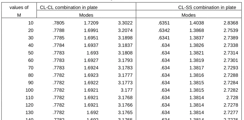
Table1.Convergence of Ω for Number of increasing nodes for CL-CL combination and CL-SS combination plates for

1, 0.4, 0.4, 0.4, 0.01, 0.01, 0.25, 0.03, 0.3,

n k k a b h v

d f

 

        

values of CL-CL combination in plate CL-SS combination in plate

M Modes Modes

10 .7805 1.7209 3.3022 .6351 1.4038 2.8368

20 .7788 1.6991 3.2074 .6342 1.3868 2.7539

30 .7785 1.6951 3.1898 .6341 1.3837 2.7389

40 .7784 1.6937 3.1837 .634 1.3826 2.7338

50 .7783 1.693 3.1808 .634 1.3821 2.7314

60 .7783 1.6927 3.1793 .634 1.3819 2.7301

70 .7783 1.6924 3.1783 .634 1.3817 2.7293

80 .7782 1.6923 3.1777 .634 1.3816 2.7288

90 .7782 1.6922 3.1773 .634 1.3815 2.7284

100 .7782 1.6921 3.177 .634 1.3815 2.7282

110 .7782 1.6921 3.1768 .634 1.3814 2.728

120 .7782 1.6921 3.1766 .634 1.3814 2.7278

130 .7782 1.692 3.1765 .634 1.3814 2.7277

140 .7782 1.692 3.1765 .634 1.3814 2.7276

Fig.1(a) Fig.1(b)

Fig.1 (a) & (b) % error in Ω for (i) CL-CL combination (ii) CL-SS combination, for α=0.4, =0.4,

k

_f



0.01,

k

_d



0.01

: □first mode; ○ second mode; ◊ third mode.

Table 1 express convergence of different modes of frequency parameters Ω with increment in number of nodes for particular parameters combinations given as: α=0.4,

0.01,

f

k





=0.04,

k

_d



0.01

for this a MATLAB coding was developed & calculation were completed for

10(10)140.

m



It was further observed that Ω for the 3 modes converges as number of nodes m increases; i.e. convergence of Ω as number of nodes increases is monotonic for both plate combinations. % error in Ω for first 3 modes of vibrations of plates is depicted in fig. 1(a) &1(b).

(5)

parameters are not zero then results compares well with Gupta M. [15], who have studied this combination with Frobenious method.

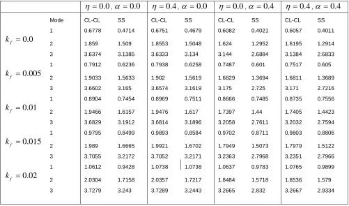
Table 2(a) and 2(b) shows the numerical results of Ω for different value of taper parameters (α) for non-damped (

0.0

d

k



) & damped (

k

d



0.01

) for two BC’s CL-CL

position and CL-SS position. The results obtained are depicted by fig. 2(a), 2(b) and 2(c) assuming fixed values of non- homogeneity parameter (



) and foundation parameters (FP) for first 3 mode of vibration of plate

combinations (i.e. CL-CL combination and CL-SS combination). Fig. 2(a) represents variation in Ω with represent to taper constant for 1st mode of Ω. We find that the value of Ω decreases as the value of α increase but introduction of foundation parameter

k

f



0.01

increase

the value of Ω for CL-SS combinations as value of taper constant increase. Fig. 2(b) represents that value of frequency parameters Ω decreases for second mode as the value of taper constant increases. The same is the nature depicted by fig. 2(c) for third mode of Ω when taper constant increases but the changes in C-C plate combination for the combination

k

_d



0.0,





0.4,

0.0

f

k



and

k

_d



0.0,





0.4,

k

_f



0.01

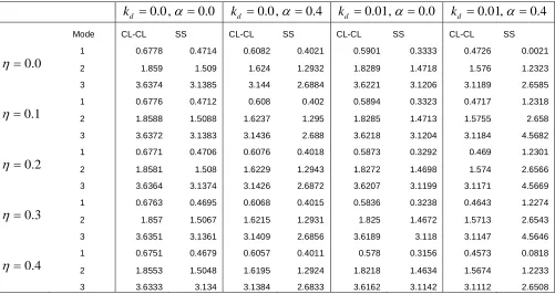
when taper constant is increases irregular.

Table 3(a) and 3(b) provided the inference that numerical value of Ω increased with the increase for different values of foundation parameters for non-damped and damped plates. Considering two different value of and α also from fig. 3(a) observed that there is parabollically increment in frequency parameter for first mode of Ω. From fig. 3(b) we observe that the increment in frequency parameters Ω with

respect to increasing foundation parameter is linear. The same is the result for third modes of Ω as for the second mode which is given by fig. 3(c) but the linear change is less in third mode then in second mode.

Table 4(a) and 4(b) provide the inference that the numerical value of Ω decreases when there is increases in the damping parameter for homogeneous and non-homogeneous plate considering two different values α and FP. From fig. 4(a) we observed that there is parabollically decrement in frequency parameters for first mode of Ω. From fig. 4(b) and 4(c) we observed that the value of frequency parameters Ω decreases linearly with increase in the value of damping parameter considering two different combination of α& FP for homogeneous and

non-homogeneous plates. Also it is observed that the linear change in second mode is much greater then third mode of frequency parameters.

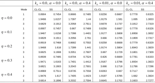
Table 5(a) and 5(b) provides the values of Ω as there is increase in values of non-homogeneity parameter Ƞ for

0.0

f

k



and

k

_f



0.01

respectively for both BC’s. The results obtained in these tables are plotted in fig. (5a), (5b) and (5c) assuming the constant value of damping parameter (

k

_d) and taper constant (



) for 3 modes of vibrations of CL-CL combination & C-SS combination. The fig. (5a), (5b) and (5c) represent the behavior of frequency parameters Ω and it decreases as there is increases in value of



for different value, taking





0.0

, 0.4 and

0.0, 0.01

d

k



& considering

k

_f as 0.0 and 0.01. Thus we observed that there is linear relationship between Ω and Ƞ for the 3 modes of CL-CL & CL-SS Plates, also the linear change is very small.

Table 2(a): Value of Ω considering different value of α, when h=0.03, ν=0.3, n=1,

k

d



0.0,

a b

/



0.25 0.0,

k

_f

0.0 







0.4,

k

_f



0.0 



0.0,

k

_f



0.01 



0.4,

k

_f



0.01

Mode CL-CL SS CL-CL SS CL-CL SS CL-CL SS

1 0.6778 0.4714 0.8904 0.7454 0.6751 0.4597 0.8969 0.7511

α=0.0 2 1.859 1.509 1.9466 1.6157 1.8553 1.4686 1.9476 1.617

3 3.6374 3.1385 3.6829 3.1912 3.5377 3.0529 3.5845 3.1896

1 0.6632 0.4599 0.8848 0.7465 0.6456 0.4494 0.8911 0.7528

α=0.1 2 1.8074 1.4645 1.9003 1.578 1.7585 1.4259 1.9007 1.5796

3 3.5264 3.0394 3.5749 3.0956 3.5216 2.9572 3.573 3.094

1 0.6469 0.4451 0.8789 0.748 0.6438 0.4359 0.8852 0.754

α=0.2 2 1.752 1.415 1.8506 1.5367 1.7471 1.3783 1.8061 1.5355

3 3.4082 2.9326 3.4603 2.9932 3.3162 2.8542 3.3697 2.9916

1 0.6286 0.4263 0.8727 0.7482 0.6257 0.4182 0.8793 0.7548

α=0.3 2 1.6908 1.3592 1.7973 1.491 1.6863 1.3244 1.7978 1.4931

3 3.2814 2.8165 3.3378 2.8824 3.276 2.7419 3.3353 2.8095

1 0.6082 0.4021 0.867 0.7485 0.6057 0.4011 0.8735 0.7556

α=0.4 2 1.624 1.2932 1.7397 1.44 1.6195 1.2914 1.7405 1.4423

(6)

1528

Table 2(b):Value of Ω considering different value of α,when h=0.03, ν=0.3, n=1,

k

_d



0.01,

a b

/



0.25 0.0,

k

f

0.0 







0.4,

k

f



0.0 



0.0,

k

f



0.01 



0.4,

k

f



0.01

1 0.5901 0.3333 0.8256 0.6667 0.578 0.3156 0.8263 0.667

α=0.0 2 1.8289 1.4718 1.9179 1.581 1.8218 1.4634 1.9157 1.5785

3 3.6221 3.1206 3.6678 3.1737 3.6162 3.1142 3.6645 3.1702

1 0.5677 0.3031 0.8156 0.6616 0.5544 0.2846 0.8159 0.6624

α=0.1 2 1.7743 1.4233 1.8688 1.5398 1.7665 1.415 1.866 1.5375

3 3.5095 3.0197 3.5583 3.0763 3.5029 3.0129 3.5543 3.0726

1 0.5414 0.2607 0.8044 0.6546 0.5273 0.2405 0.8045 0.6557

α=0.2 2 1.7148 1.3685 1.8155 1.494 1.7065 1.3602 1.8128 1.4919

3 3.3893 2.9104 3.4417 2.9715 3.3822 2.9034 3.4373 2.9677

1 0.5103 0.1953 0.7918 0.6451 0.4956 0.1691 0.7921 0.6465

α=0.3 2 1.6493 1.3058 1.7583 1.4424 1.6407 1.2972 1.7552 1.4404

3 3.2599 2.791 3.317 2.8575 3.2524 2.7837 3.3121 2.8535

1 0.4726 0.0021 0.7778 0.6325 0.4573 .0012 0.7782 0.634

α=0.4 2 1.576 1.2323 1.695 1.3883 1.5676 1.2233 1.692 1.3814

3 3.1189 2.6585 3.1812 2.7319 3.1112 2.6508 3.1765 2.7277

Table3 (a):Value of Ω considering different value of

k

_f

,

when h=0.03, ν=0.3, n=1,

k

_d



0.0,

a b

/



0.25

0.0 



,





0.0 



0.4

,





0.0 



0.0

,





0.4 



0.4

,





0.4

1 0.6778 0.4714 0.6751 0.4679 0.6082 0.4021 0.6057 0.4011

0.0

f

k



2 1.859 1.509 1.8553 1.5048 1.624 1.2952 1.6195 1.2914

3 3.6374 3.1385 3.6333 3.134 3.144 2.6884 3.1384 2.6833

1 0.7912 0.6236 0.7938 0.6258 0.7487 0.601 0.7517 0.605

0.005

f

k



₂ _1.9033 _1.5633 _1.902 _1.5619 _1.6829 _1.3694 _1.6811 _1.3689

3 3.6602 3.165 3.6574 3.1619 3.175 2.725 3.171 2.7216

1 0.8904 0.7454 0.8969 0.7511 0.8666 0.7485 0.8735 0.7556

0.01

f

k



₂ _1.9466 _1.6157 _1.9476 _1.617 _1.7397 _1.44 _1.7405 _1.4423

3 3.6829 3.1912 3.6814 3.1896 3.2058 2.7611 3.2032 2.7594 1 0.9795 0.8499 0.9893 0.8584 0.9702 0.8711 0.9803 0.8806

0.015

f

k



₂ _1.989 _1.6665 _1.9921 _1.6702 _1.7949 _1.5073 _1.7979 _1.5122

3 3.7055 3.2172 3.7052 3.2171 3.2363 2.7968 3.2351 2.7966 1 1.0612 0.9428 1.0738 1.0738 1.0637 0.9783 1.0765 0.9899

0.02

f

k



₂ _2.0304 _1.7158 _2.0357 _1.7217 _1.8484 _1.5718 _1.8536 _1.579

(7)

Table3 (b):Value of Ω consideringdifferent value of

k

_f

,

whenh=0.03, ν=0.3, n=1,

k

_d



0.01

,

a b

/



0.25 0.0,

k

f

0.0 







0.4,

k

f



0.0 



0.0,

k

f



0.01 



0.4,

k

f



0.01

1 0.5901 0.3333 0.578 0.3156 0.4726 0.0021 0.4573 0.0012

0.0

f

k



2 1.8289 1.4718 1.8218 1.4634 1.576 1.2323 1.5674 1.2233

3 3.6221 3.1208 3.6162 3.1142 3.1189 2.6585 3.1112 2.6508

1 0.7176 0.5271 0.713 0.5218 0.6436 0.4475 0.6383 0.4434

0.005

f

k



2 1.8739 1.5273 1.8693 1.5221 1.6366 1.3099 1.6309 1.3047

3 3.645 3.1474 3.6404 3.1423 3.1502 2.6954 3.144 2.6895

1 0.8256 0.6667 0.8263 0.667 0.7778 0.6325 0.7782 0.634

0.01

f

k



₂ _1.9179 _1.581 _1.9157 _1.5785 _1.695 _1.3833 _1.692 _1.3814

3 3.6678 3.1737 3.6645 3.1702 3.1812 2.7319 3.1765 2.7277

1 0.921 0.7818 0.9258 0.7858 0.8919 0.7742 0.8965 0.7791

0.015

f

k



₂ _1.9608 _1.6328 _1.9609 _1.633 _1.7515 _1.4531 _1.751 _1.4541

3 3.6905 3.1999 3.6884 3.1978 3.2119 2.7679 3.2087 2.7654 1 1.0075 0.8819 1.0156 0.8889 0.9929 0.8935 1.0009 0.901

0.02

f

k



₂ _2.0029 _1.6831 _2.0052 _1.6858 _1.8062 _1.5198 _1.8082 _1.5234

3 3.713 3.2258 3.7122 3.2251 3.2424 2.8035 3.2405 2.8026

Table4 (a): Value of Ω considering different value of

k

_d_, when h=0.03, ν=0.3, n=1,





0.0,

a b

/



0.25 0.0 ,

0.0

f

k







k

_f



0.01 ,





0.0 k

_f



0.0 ,





0.4 k

_f



0.01 ,





0.4

1 0.6778 0.4714 0.8904 0.7454 0.6082 0.4021 0.8666 0.7485

kd=0.0 2 1.859 1.509 1.9466 1.6157 1.624 1.2952 1.7397 1.44

3 3.6374 3.1385 3.6829 3.1912 3.144 2.6884 3.2058 2.7611

1 0.6726 0.464 0.8864 0.7407 0.6006 0.3893 0.8613 0.7418

kd=0.0025 2 1.8572 1.5067 1.9448 1.6136 1.621 1.2913 1.737 1.4365

3 3.6364 3.1374 3.682 3.1901 3.1424 2.6866 3.2043 2.7593

1 0.657 0.441 0.8746 0.7265 0.5773 0.3484 0.8453 0.7213

kd=0.005 2 1.8516 1.4998 1.9395 1.6071 1.6121 1.2797 1.7287 1.426

3 3.6336 3.1341 3.6792 3.1868 3.1377 2.681 3.1997 2.7539

1 0.63 0.3997 0.8545 0.7022 0.5362 0.2662 0.8179 0.6858

kd=0.0075 2 1.8421 1.4882 1.9305 1.5963 1.5972 1.2601 1.7147 1.4084

3 3.6288 3.1286 3.6744 3.1814 3.1299 2.6716 3.192 2.7447

1 0.5901 0.3333 0.8256 0.6667 0.4726 0.0021 0.7778 0.6325

kd=0.01 2 1.8289 1.4718 1.9179 1.581 1.576 1.2323 1.695 1.3833

(8)

1530

Table 4(b): Value of Ω considering different value of

k

_d

,

when h=0.03, ν=0.3, n=1,





0.4,

a b

/



0.25

.

0.0 ,

0.0

f

k







k

_f



0.01 ,





0.0 k

_f



0.0 ,





0.4 k

_f



0.01 ,





0.4

1 0.6751 0.4679 0.8969 0.7511 0.6057 0.4011 0.8735 0.7556

kd=0.00 2 1.8553 1.5048 1.9476 1.617 1.6195 1.2924 1.7405 1.4423

3 3.6333 3.134 3.6814 3.1896 3.1384 2.6833 3.2032 2.7594

1 0.6694 0.4599 0.8927 0.7461 0.5975 0.3877 0.8679 0.7486

kd=0.0025 2 1.8532 1.5022 1.9456 1.6146 1.6163 1.2873 1.7375 1.4385

3 3.6322 3.1328 3.6803 3.1884 3.1367 2.6813 3.2015 2.7574

1 0.6522 0.4348 0.8798 0.731 0.5722 0.3442 0.8507 0.7271

kd=0.005 2 1.847 1.4946 1.9396 1.6074 1.6066 1.2747 1.7285 1.4273

3 3.629 3.1291 3.6772 3.1848 3.1316 2.6752 3.1965 2.7515

1 0.6232 0.3896 0.8579 0.7051 0.5274 0.2557 0.7904 0.6899

kd=0.0075 2 1.8365 1.4817 1.9297 1.5955 1.5904 1.2536 1.6988 1.4083

3 3.6237 3.1229 3.6719 3.1787 3.1231 2.665 3.1804 2.7416

1 0.578 0.3156 0.8263 0.667 0.4573 0.0012 0.7117 0.634

kd=0.01 2 1.8218 1.4634 1.9197 1.5785 1.5674 1.2233 1.662 1.3824

3 3.6162 3.1142 3.6645 3.1702 3.1112 2.6508 3.1603 2.7277

Table 5(a): Value of Ω considering different value of



,

when h=0.03, ν=0.3, n=1,

k

_f



0.0,

a/b=0.25

k

d



0.0 ,





0.0 k

d



0.0 ,





0.4 k

d



0.01,





0.0 k

d



0.01,





0.4

1 0.6778 0.4714 0.6082 0.4021 0.5901 0.3333 0.4726 0.0021

0.0 



₂ _1.859 _1.509 _1.624 _1.2932 _1.8289 _1.4718 _1.576 _1.2323

3 3.6374 3.1385 3.144 2.6884 3.6221 3.1206 3.1189 2.6585

1 0.6776 0.4712 0.608 0.402 0.5894 0.3323 0.4717 1.2318

0.1 



₂ _1.8588 _1.5088 _1.6237 _1.295 _1.8285 _1.4713 _1.5755 _2.658

3 3.6372 3.1383 3.1436 2.688 3.6218 3.1204 3.1184 4.5682

1 0.6771 0.4706 0.6076 0.4018 0.5873 0.3292 0.469 1.2301

0.2 



₂ _1.8581 _1.508 _1.6229 _1.2943 _1.8272 _1.4698 _1.574 _2.6566

3 3.6364 3.1374 3.1426 2.6872 3.6207 3.1199 3.1171 4.5669

1 0.6763 0.4695 0.6068 0.4015 0.5836 0.3238 0.4643 1.2274

0.3 



₂ _1.857 _1.5067 _1.6215 _1.2931 _1.825 _1.4672 _1.5713 _2.6543

3 3.6351 3.1361 3.1409 2.6856 3.6189 3.118 3.1147 4.5646

1 0.6751 0.4679 0.6057 0.4011 0.578 0.3156 0.4573 0.0818

0.4 



₂ _1.8553 _1.5048 _1.6195 _1.2924 _1.8218 _1.4634 _1.5674 _1.2233

3 3.6333 3.134 3.1384 2.6833 3.6162 3.1142 3.1112 2.6508

(9)

Table 5(b): Value of Ω considering different value of



,

when h=0.03, ν=0.3, n=1,

k

_f



0.01,

a b

/



0.25

,

k

d



0.0 ,





0.0 k

d



0.0 ,





0.4 k

d



0.01,





0.0 k

d



0.01,





0.4

1 0.8904 0.7454 0.8666 0.7485 0.8256 0.6667 0.7778 0.6325

0.0 



₂ _1.9466 _1.6157 _1.7397 _1.44 _1.9179 _1.581 _1.695 _1.3833

3 3.6829 3.1912 3.2058 2.7611 3.6678 3.1737 3.1812 2.7319

1 0.8907 0.7457 0.867 0.7489 0.8256 0.6667 0.7778 0.6326

0.1 



₂ _1.9467 _1.6158 _1.7398 _1.4401 _1.9177 _1.5808 _1.6958 _1.3832

3 3.6828 3.1911 3.2056 2.761 3.666 3.1735 3.1809 2.7317

1 0.8919 0.7468 0.8682 0.7502 0.8258 0.6668 0.7779 0.6329

0.2 



₂ _1.9468 _1.616 _1.7399 _1.441 _1.9174 _1.5804 _1.6943 _1.3829

3 3.6825 3.1908 3.2051 2.7607 3.667 3.1729 3.1801 2.7309

1 0.8939 0.7485 0.8704 0.7524 0.826 0.6669 0.7781 0.6333

0.3 



₂ _1.9471 _1.6163 _1.7401 _1.4412 _1.9167 _1.5796 _1.6934 _1.3823

3 3.6821 3.1903 3.2043 2.7601 3.666 3.1718 3.1786 2.7296

1 0.8969 0.7511 0.8735 0.7556 0.8263 0.667 0.7117 0.634

0.4 



₂ _1.9476 _1.617 _1.7405 _1.4423 _1.9197 _1.5785 _1.662 _1.3824

3 3.6814 3.1896 3.2032 2.7594 3.6645 3.1702 3.1603 2.7277

Fig.2: Graphic representation of Ω considering CL-CL and CL-SS combinations in plates: (2a) I-mode (2b) II-mode (2c) III-mode, for a/b=0.25. —, C-C, ---, C-SS, *,

k

_d



0.0

,

k

_f



0.0,





0.0

;



,

k

_d



0.0

,

k

_f



0.01,





0.0

; v ,

k

_d



0.0

,

k

_f



0.0,





0.4

;



,

k

_d



0.0

,

0.01,

0.4

f

k







; ⌂,

k

_d



0.01,

k

_f



0.0,





0.0

; ꙳,

k

_d



0.01,

k

_f



0.01,





0.0

; ○,

k

_d



0.01,

0.0,

0.4

f

k







; □,

k

_d



0.01,

k

_f



0.01,





0.4

(10)

1532

Fig.3: Graphic representation of Ω considering CL-CL and CL-SS combination of plates: (3a) I-mode (3b) II-mode (3c) III-mode,

a b

/



0.25

—, C-C, ---, C-SS, *,

k

_d



0.0

,





0.0,





0.0

;



,

k

_d



0.0

,





0.0,





0.4

; v ,

k

_d



0.0

,





0.4,





0.0

;



,

k

_d



0.0

,

0.4,

0.4 







; ⌂,

k

_d



0.01,





0.0,





0.0

; ꙳,

k

_d



0.01,





0.0,





0.4

; ○,

k

_d



0.01,





0.4,





0.0

; □,

0.4,





k

_d



0.01,

0.4

Fig.(3a) Fig.(3b) Fig. (3c)

Fig.4: Graphic representation of Ωconsidering CL-CL and CL-SS combinations inplates: (4a) I- mode (4b) II- mode (4c) III-mode,

a b

/



0.25

—, CL-CL, ---, CL-SS, *,

k

_d



0.0

,

k

_f



0.0,





0.0

;



,

k

_d



0.0

,

k

_f



0.01,





0.0

; v ,

k

_d



0.0

,

k

_f



0.0,





0.4

;



,

0.0

d

k



,

k

_f



0.01,





0.4

; ⌂,

k

_d



0.01,

k

_f



0.0,





0.0

; ꙳,

k

_d



0.01,

k

_f



0.01,





0.0

; ○,

k

_d



0.01,

0.0 ,

0.4

f

k







; □,

k

_d



0.01,

k

_f



0.01,





0.4

(11)

Fig.5: Graphicrepresentation of Ω considering CL-CL and CL-SS combinations in plates: (5a) I- mode (5b) II- mode (5c) III- mode, for

a b

/



0.25

. — , CL-CL plates , ---, CL-SS, *,

k

_d



0.0

,

k

_f



0.0,





0.0

;



,

k

_d



0.0

,

k

_f



0.01,





0.0

; v ,

k

_d



0.0

,

0.0,

0.4

f

k







;



,

k

_d



0.0

,

k

_f



0.01,





0.4

; ⌂,

k

_d



0.01,

k

_f



0.0,





0.0

; ꙳,

k

_d



0.01,

0.0

f

k







; ○,

k

_d



0.01,

k

_f



0.0,





0.4

; □,

k

_d



0.01,

k

_f



0.01,





0.4

Fig.(5a) Fig.(5b) Fig. (5c)

5. CONCLUSION

For the computation of results for present problem MATLAB is used within allowed range of plate parameters as per desired accuracy

 

10

8 , it helps in validation of actual vibrational problem. The present model results deals with the effect of damping on rectangular plate considering varying thickness, thermally induced non-homogeneity and plate which rest on wrinkle type elastic foundation material using the method quintic spline interpolation technique. Determination of natural frequency of plates is of great importance in industry because plate failure can results in loss of money and life. Thus assessment of failure life of a plate structure with effect of different parameters is of most importance. Calculation of natural frequency considering the effect of different parameters helps in assessment of design of plate to engineering who can modified plate structures as per the structural need to prevent cyclic fatigue and complete failure. Thus the present model results will be greatly useful for design to civil and mechanical engineers in various industries to obtain desired frequency by controlling different parameters which in turnalso helps in robustness of the design structures.

6. REFERENCES

[1] Crandall S.H., The role of damping in vibration theory. J. of Sound and Vibration, Vol. 11, No. 1, pp. 3-18 (1970).

[2] Gupta U.S. and Lal R., Transverse Vibration of Non-uniform rectangular plate on elastic Foundation,

Journal of sound and vibration, Vol. 61, No.1, pg. 127-133, (1978).

[3] Leissa A. W., The free vibration of rectangular plates, J sound and vibrations, vol. 31 (3), pg. 257-293,(1973).

[4] Lal R., Gupta U. S., and Reena, Quintic spline in the study of transverse vibrations of non-uniform orthotropic rectangular plates. Journal of sound and vibration 207: 1-13(1997)

[5] Gupta A.K. and Jain M., Exponential temperature effect on frequencies of a rectangular plate of non- linear varying thickness. A quintic spline technique, Journal of Theoretical and Applied Mechanics, Vol. 52, No. 1, pp. 15-24, (2014).

[6] Chakraverty S., Pradhan KK., Free vibration of exponential functionally graded rectangular plates in thermal environment with general boundary conditions. Aerospsci Technol; 36:132-56, (2004).

[7] Robin and Rana U.S., Study of damped vibration of non- homogeneous rectangular plate of variable thickness, International Journal of Engineering and applied science (IJEAS), ISSN: 2394-3661, Volume-3, Issue-8, (2016).

[8] Sakata T., A note on nodal lines of rectangular plates. J. Appl. Mech., Vol. 45(3), pp. 691-693, (1978). [9] Gupta A.K., Johri T. and Vats R.P., Thermal effect on

(12)

1534 San-Francisco, USA, 24-26 Oct., 2007, pp. 784-787,

(2007).

[10] Bahmyari E. and Rahbar-Ranji A., Free vibration analysis of orthotropic plates with variable thickness resting on non-uniform elastic foundation by element free Galerkin method. Journal of Mechanical Science and Technology, vol. 26, pg. 2685-2694, (2012). [11] Sharma S., Gupta U. S., and Singhal P., Vibration

analysis of non- homogeneous orthotropic rectangular plates of variable thickness resting Winkler foundation, Journal of applied science and engineering, vol. 15(3), pp. 291-300, (2012).

[12] Tomar J.S. and Gupta A.K., Thermal gradient on frequency of orthotropic rectangular plate whose thickness varies in two directions. Journal of Sound and Vibration, Vol. 98, No. 2, pp. 257-262, (1985). [13] Gupta M., Kumar A., Kumar A., Analysis of Damping

and Non-homogeneity through spline interpolation technique of an isotropic Rectangular plate of Parabollically varying thickness which rests on Elastic foundation, ESSENCE Int. J. Env. Rehab. Conserv. X (1): 15—24(2019).ISSN : 0975 – 6272

[14] Jain R. K. and Soni S. R., Free vibration of rectangular plates of parabollically varying thickness, Indian Journal of Pure and Applied Mathematics, Vol.4(3), pp. 267-277, (1973).