Volume 2009, Article ID 248581,16pages doi:10.1155/2009/248581
Research Article
Triangular Wavelets: An Isotropic Image Representation with
Hexagonal Symmetry
Kensuke Fujinoki and Oleg V. Vasilyev
Department of Mechanical Engineering, University of Colorado, 427 UCB, Boulder, CO 80309, USA
Correspondence should be addressed to Kensuke Fujinoki,[email protected]
Received 19 May 2009; Accepted 14 September 2009
Recommended by James Fowler
This paper introduces triangular wavelets, which are two-dimensional nonseparable biorthogonal wavelets defined on the regular triangular lattice. The construction that we propose is a simple nonseparable extension of one-dimensional interpolating wavelets followed by a straightforward generalization. The resulting three oriented high-pass filters are symmetrically arranged on the lattice, while low-pass filters have hexagonal symmetry, thereby allowing an isotropic image processing in the sense that three detail components are distributed uniformly. Applying the triangular filter to images, we explore applications that truly benefit from the triangular wavelets in comparison with the conventional tensor product transforms.
Copyright © 2009 K. Fujinoki and O. V. Vasilyev. This is an open access article distributed under the Creative Commons Attribution License, which permits unrestricted use, distribution, and reproduction in any medium, provided the original work is properly cited.
1. Introduction
Image processing is one of the most demanded areas of signal processing applications, where the wavelet transform has been offered significant performance advantages [1]. In most cases, the wavelet transform is carried out in the tensor product form, that is, by applying a one-dimensional transform repeatedly in the horizontal and vertical direc-tions. This gives the simple two-dimensional extension of wavelet transforms and yields the lower-resolution images consisting of the approximation and three detail components that contain directional information. In the case of this separable transform, however, the diagonal detail component is only the product of horizontal and vertical details. Thus, isotropy in the sense of uniform distribution of three detail components may not be well respected.
To remedy this drawback many attempts have been carried out to construct nonseparable wavelets [2, 3] or to implement dual-tree complex wavelet transform [4,5], though the constructions of the associated filters are highly involved and computationally complex. The largest bottle-neck is the lack of intrinsically two-dimensional wavelets that are easy to use.
On the other hand, in the framework of subdivision scheme, the wavelet transforms on more general data sets
such as geometric meshes or surfaces have been successfully implemented [6,7]. In particular, with the advent of lifting scheme [8], the so-called second generation wavelets [9] have opened a way to handle data on irregular grids over arbitrary surfaces [10, 11]. Their main aim is, however, the efficient representation of large data sets and isotropy and/or rotational symmetry in two-dimensional data are not a major concern. If we limit to data on a plane such as images, the usual first generation wavelets would be more desirable, since they would allow more general treatments due to their periodicity on the plane.
In this context a new class of wavelets, called triangular wavelets, whose nonseparable biorthogonal filters are defined on a regular triangular lattice have recently been proposed [12]. Our formulation is based on a straightforward general-ization of one-dimensional settings including the lifting. This allows the simple nonseparable extension of biorthogonal wavelets without loosing their special properties such as vanishing moments, which are a crucial criterion for both stability and smoothness of wavelets.
are expected to improve smoothness characteristics of low-order triangular filters discussed in [13]. In addition we have observed that the energy of decomposed images is evenly distributed over the three detail components. This suggests that the triangular wavelets are promising in keeping isotropy of images, which has been a key issue in wavelet-based image processing.
As an interpolation technique, we use the Lagrange interpolation, which is a standard method of a pointwise polynomial interpolation [14]. Whereas B-splines are also known to have good approximation orders, the Lagrangian method allows us to construct interpolating wavelets having any number of vanishing moments [15]. Unlike in the case of splines, their coefficients are given by easy explicit formulas, and the associate functions are an optimal tradeoff between support size and approximation order, in a similar way to Daubechies wavelets [16]. Moreover, the wavelet transform with any order of the interpolating filters can be implemented by only two lifting steps. This remarkable fact would be quite important in our direct generalization scheme.
It should be noted that orthogonal quadrature mirror filters and biorthogonal wavelets defined on the triangular lattice have also been considered [17–19]. While their formulations partially agree with ours, one of the crucial differences is that their filter construction relies on the numerical analysis technique or algebraic approaches. In contrast, our method uses direct generalization of lifting and, thus, resulting in easy construction of biorthogonal wavelet filters or perfect reconstruction filters. In addition to low computational cost of the triangular wavelet transform, the filter coefficients are all rational numbers.
This paper is organized as follows. Section 2 briefly reviews the one-dimensional wavelets including the lifting scheme and interpolating wavelets. The two-dimensional nonseparable biorthogonal wavelets on triangular lattice are developed inSection 3. The application of triangular wavelet transform to image analysis and performance comparison with conventional tensor product wavelets are given in
Section 4. Finally, conclusions are drawn inSection 5.
2. Biorthogonal Wavelets
2.1. Perfect Reconstruction Filters. The wavelet transform decomposes a signal cj[k], j,k ∈ Z into the coarse
componentcj−1[k] and detail componentdj−1[k] by a
low-pass (LP) filterh[k] and a high-pass (HP) filterg[k] followed by subsampling. In the Fourier domain, the signal is defined by
cj(ω)=
k∈Z
cj[k]e−iωk, ω∈R, (1)
and the decomposition is written as
⎛
⎝cj−1(2ω)
dj−1(2ω) ⎞ ⎠=1
2M ∗(ω)
⎛ ⎝ cj(ω)
cj(ω+π) ⎞
⎠, (2)
whereM∗(ω) is the complex conjugate of the modulation matrix
M(ω)=
⎛
⎝h(ω) h(ω+π)
g(ω) g(ω+π)
⎞
⎠. (3)
Here, we assume that h(0) = √2 and g(0) = 0. The reconstruction of the original signal is carried out by taking the reverse steps using the dual filtersh[k] andg[k], which may be written as
⎛ ⎝ cj(ω)
cj(ω+π) ⎞
⎠=MT(ω)
⎛
⎝cj−1(2ω)
dj−1(2ω) ⎞
⎠, (4)
whereM(ω) is the transpose of the dual modulation matrix defined similarly as (3). The exact reconstruction of the original signal from the decomposition is guaranteed if the filters satisfy the perfect reconstruction condition
M
T
(ω)M∗(ω)=2I. (5)
Such particular filters are called perfect reconstruction filters or biorthogonal filters that satisfy the biorthogonality condition derived from (5)
h(ω)h∗(ω) +g(ω)g∗(ω)=2,
h(ω)h∗(ω+π) +g(ω)g∗(ω+π)=0,
(6)
with
g(ω)=e−iωh ∗
(ω+π), g(ω)=e−iωh∗(ω+π). (7)
Once a set of biorthogonal filters are devised, the associated scaling functionsφand waveletsψare defined by
φ(ω)=√1
2h
ω 2
φ
ω 2
, ψ(ω)=√1
2g
ω 2
φ
ω 2
,
(8)
whose inverse Fourier transforms yield the particular rela-tions
φ(t)=
k∈Z
√
2h[k]φ(2t−k),
ψ(t)=
k∈Z
√
2g[k]φ(2t−k).
(9)
Their dual functions are also defined by using dual filters in a similar way which, together with the primal pair, turn out to form an biorthogonal basis forL2(R).
We now move to the polyphase domain to introduce the lifting scheme for construction of biorthogonal wavelet filters. In the polyphase representation, a signal cj[k] is
defined in terms of its even and odd components separately
cj,e(ω)=
k∈Z
cj[2k]e−iωk, cj,o(ω)=
k∈Z
cj[2k+ 1]e−iωk.
We then have the relation
⎛ ⎝ cj(ω)
cj(ω+π) ⎞
⎠=U(ω)
⎛ ⎝cj,e(2ω)
cj,o(2ω) ⎞
⎠, (11)
where
U(ω)=
⎛
⎝1 e−iω
1 e−i(ω+π) ⎞
⎠. (12)
With the polyphase form of an LP filter h[k] and an HP filterg[k] defined similary as (10), we assemble the polyphase matrix as
P(ω)=
⎛
⎝he(ω) ge(ω)
ho(ω) go(ω) ⎞
⎠, (13)
so that
P(2ω)†=1
2M
∗(ω)U(ω), (14)
where P(ω)† is the Hermitian conjugate of the polyphase matrix. The modulation matrix can also be found from the polyphase matrix
MT(ω)=U(ω)P(2ω). (15)
In the polyphase domain, decomposition (2) and the reconstruction (4) may be rewritten as
⎛ ⎝cj−1(ω)
dj−1(ω) ⎞
⎠=P(ω)†
⎛ ⎝cj,e(ω)
cj,o(ω) ⎞ ⎠,
⎛ ⎝cj,e(ω)
cj,o(ω) ⎞ ⎠=P(ω)
⎛ ⎝cj−1(ω)
dj−1(ω) ⎞ ⎠,
(16)
whereP(ω) is the dual polyphase matrix formed similarly as (13) with dual filtershandg. Then the perfect reconstruction condition (5) becomes
P(ω)P(ω)†=I. (17)
Thus, finding the perfect reconstruction filters (h,h,g,g) amounts to find P(ω)† and P(ω) that satisfy (17). This condition implies that the matrices must be invertible, and the inverse should be polynomials ofe±iω, which provides
perfect reconstruction FIR filters and thus compactly sup-ported wavelets.
2.2. Lifting Scheme. Lifting is a convenient method to con-struct an invertible polyphase matrix. The odd component cj[2k + 1] is predicted by a predictor p using the even
component cj[2k], and cj[2k + 1] is replaced by dj−1[k]
which is the differences between the original values and the prediction at the odd indices
cj[2k+ 1]−→dj−1[k]=cj[2k+ 1]−p
cj[2k]
. (18)
The even componentcj[2k] is then updated using the results
of the prediction
cj[2k]−→cj−1[k]=cj[2k] +u
dj−1[k]
, (19)
where the updater u is designed so that the coarse signal preserves the average of the original signal
k
cj−1[k]=
1 2
k
cj[k]. (20)
Note the fact that the computation in these two steps can be performed in-place, which reduces computational cost of the wavelet transform. Finally,cj−1[k] anddj−1[k] are scaled
by K and 1/K, respectively, for the energy normalization
cj[k]2= cj−1[k]2+dj−1[k]2.
Each lifting step corresponds to the factorization of the polyphase matrix
P(ω)†=
⎛ ⎜ ⎝
K 0
0 1
K
⎞ ⎟ ⎠ ⎛ ⎝1 u(ω)
0 1
⎞ ⎠ ⎛
⎝ 1 0
−p(ω) 1
⎞
⎠, (21)
where p(ω) is defined by kp(cj[k])e−iωk = p(ω)cj(ω),
and similarly for the updater u(ω). One can immediately recognize that these factorized matrices are all invertible, and hence it is easy to construct the dual polyphase matrix by taking its inverseP(ω)=P(ω)†−1.
For example, the simple choice p(ω) = 1,u(ω) = 1/2,
andK=√2 gives the orthogonal Haar filtersh(ω)=h(ω)= (1 +e−iω)/√2 and g(ω) = g(ω) = (−1 +e−iω)/√2. The
predictor operator uses the even componentcj[2k] at its left
neighboring odd componentcj[2k + 1]. The order of the
predictor is one [15]. The prediction is accurate if a signal is constant or, in other words, zeroth-order polynomial.
If we choose the linear prediction
p(ω)=1 +e−iω
2 , u(ω)=
1 +eiω
4 , (22)
andK=√2, we obtain CDF(2, 2) biorthogonal filters [20]
h(ω)= −ei2ω+ 2eiω+ 6 + 2e−iω−e−i2ω
4√2 ,
g(ω)= −1 + 2e−iω−e−i2ω
2√2 .
(23)
In this linear case, the order of the predictor is two, which predicts first-order polynomials of a signal. Both HP filters
−2
−1 0 1 2 3 4 5
−2 −1 0 1 2
φ(t)
(a)
−4
−2 0 2 4 6
−1 −0.5 0 0.5 1 1.5 2
ψ(t)
(b)
0 0.2 0.4 0.6 0.8 1
−2 −1 0 1 2
φ(t)
(c)
0 0.5 1 1.5
−1 −0.5 0 0.5 1 1.5 2
ψ(t)
(d)
Figure1: The system (φ,ψ,φ,ψ) of CDF(2, 2) biorthogonal wavelets with 2 vanishing moments.
2.3. Interpolating Wavelets. To build a higher-order pre-dictor, we use the Lagrange interpolation scheme. The corresponding interpolating filter is Lagrange half-band filter [22], which is a symmetric maxflat filter that satisfiesh(ω)=
h(−ω) and
h(ω) +h(ω+π)=√2. (24)
The filter has 2L+ 1 nonzero coefficients and is the shortest filter that reproduces mid-values of polynomials of degree 2L−1 from a given set of samples. Therefore, the Lagrange half-band filter can directly be used as a 2Lth-order predictor of the lifting scheme. For anyL ≥ 1 and−L < k ≤ L, the coefficients are given in an explicit form as
hL[2k−1]= (−1)
L+k−12L
n=1(L−n+ 1/2)
(L+k−1)!(L−k)!(k−1/2), (25)
and the even coefficients are constrained as hL[2k] =
δ[k]. They are also known to be identical to those of the Deslauriers-Dubuc filters [23,24] of orderN=2L.
When the odd coefficients of the Lth-order Lagrange half-band filter are chosen to be a predictor p[k] of order N
p[k]=pN[k]=hL[2k−1], (26)
one can set an updater as
u(ω)= pN∗(ω)
2 forN≤N. (27)
As a result, we can obtain a family of (N,N) interpolating wavelet filters constructed in [8], where (N,N) denotes the number of vanishing moments of HP filters (g,g). They are a set of symmetric biorthogonal perfect reconstruction FIR filters (h,h,g,g), wherehis equivalent to the Lagrange half-band filter (25) of order 2L=N, and the corresponding dual scaling functionφis an interpolating function that recovers polynomials of degreeN−1. It is remarkable to note that
h(ω)h ∗
(ω) in caseN=Ngives rise to the orthogonal maxflat Daubechies filter withNvanishing moments [22].
The case (N = 2, N = 2) amounts to CDF(2, 2)
filters (23) whose wavelet and scaling functions are shown in
0.5 1 1.5
0 π
4
π
2
3π
4
π
ω
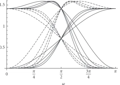
Figure 2: Frequency responses of (N,N) interpolating filters
(|h(ω)|,|h(ω)|,|g(ω)|,|g(ω)|) for even orders 2 to 8 in caseN =
N, which are obtained according to the coefficients given in
Table 1. Solid line and dashed line represent primal and dual filters, respectively. AsN andN increase, the filters are increasingly flat at ω=0 andω=π.
Table 1 shows the different orders of predictor pN[k]
based on Lagrange half-band filters defined in (26). The frequency responses of corresponding filters (h,h,g,g) are shown in Figure 2. As N and N increase, the filters are increasingly flat atω=0 andω=π, which implies that a lack of smoothness of a signal after the decomposition would be improved. Their filter coefficients are always of the formz/2n
wherez∈Z,n∈N, thereby allowing an implementation of the integer wavelet transform [25], which has been adopted in the JPEG2000 standard.
3. Triangular Biorthogonal Wavelets
This section presents triangular wavelets, which are two-dimensional nonseparable wavelets defined on a regular triangular lattice. The construction basically follows a straightforward generalization of the interpolating wavelets described before. We first study a method for generating the triangular lattice. Then we show how the filters as well as wavelets constructed inSection 2fit into the general settings.
3.1. Bravais Lattice Formalism. A discrete signal is naturally indexed by integers in one dimension, but the indexing may become a nontrivial problem in two or higher dimensions. Here we introduce a convenient method of site indexing for a two-dimensional plane by employing the primitive translation vectors. In solid state physics, possible crystals are classified as lattice structures called Bravais lattice generated by three primitive translation vectors. While general crystals have three-dimensional structures, the basic idea is still applicable in two dimension and poses no basic problems. We begin our formulation following the general strategy in solid state physics for example [26].
We define two primitive translation vectors
t1=
1 0T, t2=
−1
2
√
3 2
T
, (28)
with which the regular triangular Bravais lattice is defined by
Λ=t=n1t1+n2t2|(n1,n2)∈Z2
. (29)
The domain containing all the points whose closest site is a sitet ∈ Λis the Wigner-Seitz cell of the site, which is also called the Voronoi cell. It is the domain of definition of a function f(r),r∈R2. Each site belongs to its corresponding
Wigner-Seitz cell, and a whole planeR2 is represented as a
tiling of the cells. For a two-dimensional discrete signal such as an image, this plays the role of a pixel. In our setting the Wigner-Seitz cell is a hexagon, as shown inFigure 3.
The reciprocal lattice vectors are similarly defined by
λ1=
0 √2 3
T
, λ2=
1 √1 3
T
, (30)
which generate the reciprocal lattice
Λ=2π(λ=n1λ1+n2λ2)|(n1,n2)∈Z2
. (31)
The Wigner-Seitz cell of the reciprocal lattice Λ is called the Brillouin zone, which is also a hexagon (seeFigure 3). Analogous to the nature of the Wigner-Seitz cells, a whole
ω-plane can also be tiled by a set of Brillouin zones, as illustrated together inFigure 4.
For notational convenience we also definet0 =λ0 = 0,
t3= −t1−t2, andλ3=λ1−λ2, holding the relation
λm·tm=0, m=0, 1, 2, 3. (32)
Note that t3 and λ3 are not linearly independent and in
particular
e−iπnλi·tj = ⎧ ⎨ ⎩
1, i=j,
(−1)n, i /=j, i,j=1, 2, 3, n∈Z. (33)
A discrete signal{cj[t]}t∈Λis assumed to be given on the
Bravais latticeΛ, and its Fourier transform
cj(ω)=
t∈Λ
cj[t]e−iω·t, ω∈R2, (34)
is doubly periodic with period 2πλ
cj(ω)=cj(ω+ 2πλ), λ∈Λ. (35)
Thus, one of the Brillouin zones is the domain of definition ofcj(ω), which corresponds to the interval [−π,π] in one
dimension. In particular, the aliasing frequencies occur at the boundary of the Brillouin zones. Unlike the one-dimensional setting, where there exists only one alias point atω=π, we have three alias points atω = πλk,k = 1, 2, 3 due to the
Table1: Coefficients for predictorpN[k] of orderNbased on Lagrange interpolation.
N\k −4 −3 −2 −1 0 1 2 3 4 5 Scaling
2 1 1 /2
4 −1 9 9 −1 /24
6 3 −25 150 150 −25 3 /28
8 −5 49 −245 1225 1225 −245 49 −5 /211
10 35 −405 567 −2205 19845 19845 −2205 567 −405 35 /216
−1 1 2
−1 1 2
t2
t3
t1
y
x
(a)
−2π 2π
−2π
2π
4π
2πλ3
2πλ1
2πλ2
η
ξ
(b)
Figure3: Bravais latticeΛgenerated by two primitive translation vectorst1andt2, and Wigner-Seitz cell (a); reciprocal latticeΛgenerated
by two reciprocal lattice vectorsλ1andλ2, and Brillouin zone (b). For notational conveniencet3andλ3are also defined.
A crucial observation is that the Bravais latticeΛmay be split into four sublattices
Λm= {2t+tm|t∈Λ}, m=0, 1, 2, 3. (36)
The set Λ is now partitioned, and these four sets Λm are
completely disjointed from each other. If we add all of the sites of sublattices, then we recover the original lattice. This is exactly the polyphase decomposition of the Bravais lattice, which immediately indicates that we have four polyphase components and thus four patterns of indices (seeFigure 5). For example, a signal {cj[t]}t∈Λ is represented as its four
polyphase components
cm,j(ω)=
t∈Λ
cj[2t+tm]e−iω·t, m=0, 1, 2, 3, (37)
which play the role of even and odd indices in one dimension. Then the formula analogous to (11) is
⎛ ⎜ ⎜ ⎜ ⎜ ⎜ ⎜ ⎝
cj(ω)
cj(ω+πλ1)
cj(ω+πλ2)
cj(ω+πλ3) ⎞ ⎟ ⎟ ⎟ ⎟ ⎟ ⎟ ⎠
=U(ω)
⎛ ⎜ ⎜ ⎜ ⎜ ⎜ ⎜ ⎝
c0,j(2ω)
c1,j(2ω)
c2,j(2ω)
c3,j(2ω) ⎞ ⎟ ⎟ ⎟ ⎟ ⎟ ⎟ ⎠
, (38)
where
U(ω)=
⎛ ⎜ ⎜ ⎜ ⎜ ⎜ ⎜ ⎝
1 e−iω·t1 e−iω·t2 e−iω·t3
1 e−iω·t1 −e−iω·t2 −e−iω·t3
1 −e−iω·t1 e−iω·t2 −e−iω·t3
1 −e−iω·t1 −e−iω·t2 e−iω·t3
⎞ ⎟ ⎟ ⎟ ⎟ ⎟ ⎟ ⎠
. (39)
In order to obtain the wavelet transform applied to our triangular lattice, the filters used for the decomposition
and reconstruction must be formed by a set of four filters, because we have four polyphase components. The straight-forward generalization shows that the possible combination of four filters turns out to be one LP and three independent HP filters{h[t],g1[t],g2[t],g3[t]}t∈Λ, which satisfies
h(ω)h∗(ω) +
3
m=1
gm(ω)gm∗(ω)=4,
h(ω)h∗(ω+πλ1) + 3
m=1
gm(ω)gm∗(ω+πλ1)=0,
h(ω)h∗(ω+πλ2) + 3
m=1
gm(ω)gm∗(ω+πλ2)=0,
h(ω)h∗(ω+πλ3) + 3
m=1
gm(ω)gm∗(ω+πλ3)=0,
(40)
or in terms of the modulation matrix
M
T
(ω)M∗(ω)=4I, (41)
where
M(ω)=
⎛ ⎜ ⎜ ⎜ ⎜ ⎜ ⎜ ⎝
h(ω) h(ω+πλ1) h(ω+πλ2) h(ω+πλ3)
g1(ω) g1(ω+πλ1) g1(ω+πλ2) g1(ω+πλ3)
g2(ω) g2(ω+πλ1) g2(ω+πλ2) g2(ω+πλ3)
g3(ω) g3(ω+πλ1) g3(ω+πλ2) g3(ω+πλ3) ⎞ ⎟ ⎟ ⎟ ⎟ ⎟ ⎟ ⎠
,
y
x
(a)
η
ξ
(b)
Figure4: Set of Wigner-Seits cells (a) and Brillouin zones (b) in Bravais latticeΛand reciprocal latticeΛ, respectively. Both whole planeR2
can be represented as a tilling of them.
andM(ω) is defined in a similar way. As in one dimension, the set of these four filters produces a scaling functionφand waveletsψm,m=1, 2, 3 defined onR2
φ(ω)=1
2h
ω
2
φ
ω
2
, ψm(ω)=
1 2gm
ω
2
φ
ω
2
,
(43)
which are normalized asφ(0)=1 andψm(0)=0, assuming
thath[0]=2 andg[0]=0. Note that we have three wavelets. On the Bravais latticeΛthey satisfy the relation
φ(r)= t∈Λ
2h[t]φ(2r−t),
ψm(r)=
t∈Λ
2gm[t]φ(2r−t).
(44)
The dual scaling function and wavelets are formed similarly.
3.2. Triangular Wavelet Transform. Corresponding to the decomposition of the Bravais lattice Λ, the polyphase representation of a LP filter{h[t]}t∈Λ and three HP filters
{gk[t]}t∈Λ,k=1, 2, 3, are given by the following form:
h(ω) g1(ω) g2(ω) g3(ω) T
=
⎛ ⎜ ⎜ ⎜ ⎜ ⎜ ⎜ ⎝
h0(2ω) h1(2ω) h2(2ω) h3(2ω)
g1,0(2ω) g1,1(2ω) g1,2(2ω) g1,3(2ω)
g2,0(2ω) g2,1(2ω) g2,2(2ω) g2,3(2ω)
g3,0(2ω) g3,1(2ω) g3,2(2ω) g3,3(2ω) ⎞ ⎟ ⎟ ⎟ ⎟ ⎟ ⎟ ⎠ ⎛ ⎜ ⎜ ⎜ ⎜ ⎜ ⎜ ⎝
1
e−iω·t1 e−iω·t2
e−iω·t3
⎞ ⎟ ⎟ ⎟ ⎟ ⎟ ⎟ ⎠
,
(45)
where
hm(ω)=
t∈Λ
h[2t+tm]e−iω·t,
gk,m(ω)=
t∈Λ
gk[2t+tm]e−iω·t,
m=0, 1, 2, 3. (46)
y
x
(a)
y
x
(b)
Figure5: Polyphase decomposition of the Bravais latticeΛ(a) into four sublatticesΛm,m =0, 1, 2, 3 (b). Circle mark (a) represents original lattice sites while under side of circle, square, triangle, and star marks (b) represents each polyphase of four sublattices according to directions int0,t1,t2, andt3, respectively.
We then assemble the polyphase matrix as
P(ω)=
⎛ ⎜ ⎜ ⎜ ⎜ ⎜ ⎜ ⎜ ⎝
h0(ω) g1,0(ω) g2,0(ω) g3,0(ω)
h1(ω) g1,1(ω) g2,1(ω) g3,1(ω)
h2(ω) g1,2(ω) g2,2(ω) g3,2(ω)
h3(ω) g1,3(ω) g2,3(ω) g3,3(ω) ⎞ ⎟ ⎟ ⎟ ⎟ ⎟ ⎟ ⎟ ⎠
, (47)
and dual polyphase matrixP(ω) similarly.
4 4 4 LP HP1 HP2 HP3 4 4 4 4 4
eiω·t3
eiω·t2
eiω·t1
P(ω)† P(ω)
e−iω·t3
e−iω·t2
e−iω·t1
+
Figure 6: Poplyphase representation of triangular wavelet trans-form. First signal is decomposed into four phases subsampled by 4, then they are filtered by applying the polyphase matrix to yield the coarse (LP) and three detail (HP) components. The inverse transform is simply realized with the dual polyphase matrix by taking the exactly backward procedure.
decomposed into a coarse componentcj−1 and three detail
componentsdm,j−1,m=1, 2, 3, subsampled by a factor of 4 ⎛ ⎜ ⎜ ⎜ ⎜ ⎜ ⎜ ⎜ ⎝
cj−1(ω)
d1,j−1(ω)
d2,j−1(ω)
d3,j−1(ω) ⎞ ⎟ ⎟ ⎟ ⎟ ⎟ ⎟ ⎟ ⎠
=P(ω)†
⎛ ⎜ ⎜ ⎜ ⎜ ⎜ ⎜ ⎝
c0,j(ω)
c1,j(ω)
c2,j(ω)
c3,j(ω) ⎞ ⎟ ⎟ ⎟ ⎟ ⎟ ⎟ ⎠ , (48)
which is illustrated schematically in Figure 6. The original signalcjcan be reconstructed by the inverse transform
⎛ ⎜ ⎜ ⎜ ⎜ ⎜ ⎜ ⎝
c0,j(ω)
c1,j(ω)
c2,j(ω)
c3,j(ω) ⎞ ⎟ ⎟ ⎟ ⎟ ⎟ ⎟ ⎠
=P(ω)
⎛ ⎜ ⎜ ⎜ ⎜ ⎜ ⎜ ⎜ ⎝
cj−1(ω)
d1,j−1(ω)
d2,j−1(ω)
d3,j−1(ω) ⎞ ⎟ ⎟ ⎟ ⎟ ⎟ ⎟ ⎟ ⎠ , (49)
assuming that the perfect reconstruction condition is satis-fied
P(ω)P(ω)†=I. (50)
As we see inFigure 6, the structure of the triangular wavelet transform is essentially the same as that of a four-channel filter bank for a two-dimensional signal. On the lattice plane the decomposition and the reconstruction are defined by convolutions and subsampling of the output by 4. This can be written in terms of the extension of the Mallat algorithm [27]
cj−1[t]=
s∈Λ
h∗[s−2t]cj[s],
dm,j−1[t]=
s∈Λ
gm∗[s−2t]cj[s],
cj[t]=
s∈Λ ⎛
⎝ h[t−2s]cj−1[s] +3 m=1
gm[t−2s]dm,j−1[s] ⎞ ⎠.
(51)
Recall that the lifting scheme corresponds to the factor-ization of a polyphase matrix. It allows one to construct any biorthogonal filters as well as fast in-place implementation
of the wavelet transform that require less computational cost than the direct implementations (51). We now wish to extend the factorization (21) to our case, which is found to be
P(ω)†=
⎛ ⎜ ⎜ ⎜ ⎜ ⎜ ⎜ ⎜ ⎜ ⎜ ⎝
K 0 0 0
0 1
K 0 0
0 0 1
K 0
0 0 0 1
K ⎞ ⎟ ⎟ ⎟ ⎟ ⎟ ⎟ ⎟ ⎟ ⎟ ⎠ × ⎛ ⎜ ⎜ ⎜ ⎜ ⎜ ⎜ ⎝
1 u1(ω) u2(ω) u3(ω)
0 1 0 0
0 0 1 0
0 0 0 1
⎞ ⎟ ⎟ ⎟ ⎟ ⎟ ⎟ ⎠ ⎛ ⎜ ⎜ ⎜ ⎜ ⎜ ⎜ ⎝
1 0 0 0
−p1(ω) 1 0 0
−p2(ω) 0 1 0
−p3(ω) 0 0 1 ⎞ ⎟ ⎟ ⎟ ⎟ ⎟ ⎟ ⎠ , (52)
with three predictors pm and updaters um, m = 1, 2, 3.
Obviously, these matrices are still invertible. The lifting implementation of the triangular wavelet transform is then realized by the following steps. First, we have three predict steps; three odd componentscj[2t+tm], m = 1, 2, 3, are
predicted by three predictorspm, respectively,
cj[2t+t1]−→d1,j−1[t]=cj[2t+t1]−p1
cj[2t]
,
cj[2t+t2]−→d2,j−1[t]=cj[2t+t2]−p2
cj[2t]
,
cj[2t+t3]−→d3,j−1[t]=cj[2t+t3]−p3
cj[2t]
. (53)
Then the update step is carried out dealing with three results of the prediction
cj[2t]−→cj−1[t]=cj[2t] + 3
m=1
um
dm,j−1[t]
, (54)
which preserves the average of a two-dimensional signal. Finally the normalization steps are applied.
Since we take three predict steps, we have degrees of free-dom to design three independent HP filters. If we make the filters isotropic, the energy of three detail componentsdm,j−1
is expected to be evenly distributed while the diagonal detail component in the tensor product transform is not essentially the independent component. The factorization (52) forM -channel case is also considered in [28], where the individual predictors are modified depending on the situations. In our setting, we directly use the one-dimensional predictor for each predictorpmin (52), and its subscriptmcorresponds to
the directions of symmetric primitive translation vectorstm.
This gives much easier extension of one-dimensional filters and obtains three isotropic HP filters whose coefficients on the triangular lattice are symmetrically arranged with respect to the origin. Moreover, this trigonal arrangement of filter coefficients provides hexagonal symmetry for the LP filter if each updaterum is also set in a similar manner. We now
3.3. Triangular Interpolating Wavelets. In this section we extend (N,N) interpolating filters presented inSection 2.2
including the Haar filter to the triangular lattice using (52). As in one dimension, the simplest choice
K=2, pm(ω)=1, um(ω)= 1
4, m=1, 2, 3, (55)
and P(ω) = P(ω)†−1 gives two-dimensional Haar filters defined on the lattice, which turn out to be biorthogonal
⎛ ⎜ ⎜ ⎜ ⎜ ⎜ ⎜ ⎝
h(ω)
g1(ω)
g2(ω)
g3(ω) ⎞ ⎟ ⎟ ⎟ ⎟ ⎟ ⎟ ⎠ =1 2 ⎛ ⎜ ⎜ ⎜ ⎜ ⎜ ⎜ ⎝
1 1 1 1
−1 1 0 0
−1 0 1 0
−1 0 0 1
⎞ ⎟ ⎟ ⎟ ⎟ ⎟ ⎟ ⎠ ⎛ ⎜ ⎜ ⎜ ⎜ ⎜ ⎜ ⎝ 1
e−iω·t1
e−iω·t2 e−iω·t3
⎞ ⎟ ⎟ ⎟ ⎟ ⎟ ⎟ ⎠ , ⎛ ⎜ ⎜ ⎜ ⎜ ⎜ ⎜ ⎜ ⎜ ⎝
h(ω) g1(ω)
g2(ω) g3(ω)
⎞ ⎟ ⎟ ⎟ ⎟ ⎟ ⎟ ⎟ ⎟ ⎠ =1 2 ⎛ ⎜ ⎜ ⎜ ⎜ ⎜ ⎜ ⎝
1 1 1 1
−1 3 −1 −1
−1 −1 3 −1
−1 −1 −1 3
⎞ ⎟ ⎟ ⎟ ⎟ ⎟ ⎟ ⎠ ⎛ ⎜ ⎜ ⎜ ⎜ ⎜ ⎜ ⎝ 1
e−iω·t1 e−iω·t2
e−iω·t3
⎞ ⎟ ⎟ ⎟ ⎟ ⎟ ⎟ ⎠ . (56)
In a similar way, we generalize (N,N) interpolating filters by letting predictorspmaspmN[ktm]=pN[k], wherepN[k] is
given inTable 1and slightly rewriting condition (27) as
um(ω)=
pN∗
m (ω)
4 forN≤N. (57)
A set of resulting filters (h,h,gm,gm) is (N,N) interpolating
filters defined on the triangular lattice. Since our construc-tion is straightforward generalizaconstruc-tion of the one-dimensional case, the dual LP filterhis still interpolating or half-band in the sense that
h(ω) +
3
m=1
h(ω+πλm)=2, (58)
which is in place of (24). If we extend the linear prediction (22) according to (57)
pm(ω)=1 +e
−iω·tm
2 , um(ω)=
1 +eiω·tm
8 , (59)
withK =2, then we obtain the triangular version of (2, 2) interpolating filters or CDF(2, 2) filters. This shows that our method is general so that (N,N) interpolating filters of higher-order can be generalized directly.
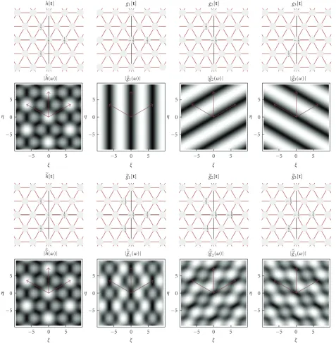
For the Haar and (2, 2) interpolating cases, we display the filter coefficients and their frequency responses with vectors 2πλm in Figures 7 and8. In each case ofm = 1, 2, 3, the
coefficients of primal HP filters gm are one dimensionally
arranged along the directions of the primitive translation vectorstm. This is true for dual filtersgmwhile they have
two-dimensional support on the lattice plane. In other words, this means that both HP filters (gm,gm) are isotropic as we exactly
intended, andm=1 andm=3 cases are thus simply 2π/3
Table2: Number of zeros for triangular (N,N) interpolating filters.
h g1 g2 g3 h g1 g2 g3
ω=πλ1 N 0 N N N N N N
ω=πλ2 N N 0 N N N N N
ω=πλ3 N N N 0 N N N N
rotations of them = 2 case. As we mentioned before, it is obvious that the triangular filters are periodic with respect to the translationω → ω+ 2πλ, and (h,h) are intrinsically two-dimensional LP filters having the hexagonal symmetry.
Let us now concentrate on the nature of the triangular filters along the directions of reciprocal lattice vectorsλm,
m=1, 2, 3. Due to the hexagonal symmetry, LP filters have the same structure for each direction ofλm. In particular, we
derive from (58) that they are also half-band
h(ωλk) +h(ωλm+πλm)=2, k,m=1, 2, 3, (60)
and the biorthogonality condition implies
h∗(ωλk)h(ωλk) +h∗(ωλm+πλm)h(ωλm+πλm)=4. (61)
Correspondingly, one-dimensional responses of three HP filters for directions in λm are defined from the LP filters
in a manner similar to (7). The relations are summarized as follows:
gk(ωλm)= ⎧ ⎪ ⎨ ⎪ ⎩
0, k=m,
1 2e
−iωtk·λmh(ωλ
m+πλm), k /=m,
gk(ωλm)= ⎧ ⎪ ⎨ ⎪ ⎩
h(ωλm+πλm), k=m,
e−iωtk·λmh(ωλ
m+πλm), k /=m,
(62)
where exponential factors give±1 according to (33). In fact,
the frequency responses of LP filters h(ωλm) and h(ωλm)
amount to the one-dimensional cases shown inFigure 2, and hence the same holds for HP filtersgk(ωλm) andgk(ωλm) in
casek /=m. Note the different normalization factor.
The HP filters (gm(ω),gm(ω)),m =1, 2, 3, have (N,N)
vanishing moments. More precisely, the vanishing moment that we consider here is the number of zeros of gm(ωλm)
and gm(ωλm) at ω = 0. Similarly LP filters h(ωλm) and
h(ωλm) have zeros atω=π, which corresponds to the alias
pointsω =πλm. The number of zeros of triangular (N,N)
interpolating filters is summarized inTable 2.
−5 0 5
η
−5 0 5
η η
−5 0 5
η
−5 0 5
η
−5 0 5
η
−5 0 5
η
−5 0 5
η
−5 0 5
η
−5 0 5
ξ
−5 0 5
ξ
−5 0 5
ξ
−5 0 5
ξ
−5 0 5
ξ
−5 0 5
ξ
−5 0 5
ξ
−5 0 5
ξ
1 2
1 2
1 2 1
2 −
1 2
−1 2
3 2
−1 2
3 2
−1
2 −
1 2
−1 2
−1 2
−1
2 −
1 2
3 2
−1
2 −
1 2 1
2
1 2
1 2
1 2
−1 2
1 2
1 2
−1 2
1 2
−1 2
h[t] g1[t] g2[t] g3[t]
|h(ω)| |g1(ω)| |g2(ω)| |g3(ω)|
h[t] g1[t] g2[t] g3[t]
|h(ω)| |g1(ω)| |g2(ω)| |g3(ω)|
Figure7: Frequency responses of triangular biorthogonal Haar filters (h,gm,h,gm),m=1, 2, 3, whose arrows indicate 2πtimes reciprocal lattice vectorsλm.
functions are identical and its value is 1 over the white region and 0 otherwise, while the wavelets have positive, zero, and negative values represented, respectively, in black, grey, and white. It is interesting to note that the scaling function with this fractal shape tiles a whole planeR2. Such functions are
also obtained in [29] on the rectangular settingt1 =(1, 0)T
and t2 = (0, 1)T as one of the particular functions that
have the property of self-similar tiling ofRn. On the other
hand, the set of (2, 2) interpolating wavelets, shown also in
Figure 9, is obviously no longer involved with a fractal shape. Their supports are based on the corresponding filters as given
in Figure 8 where LP filters h and h have the hexagonal symmetry. They are much more smooth functions but both primal functions still seem to contain jaggy parts, as we have already seen in their one-dimensional shapes shown in Figure 1. As we pointed out in Section 2, this lack of regularity is improved by increasing the order ofNandN.
4. Applications
−5 0 5 η −5 0 5 η η −5 0 5 η −5 0 5 η −5 0 5 η −5 0 5 η −5 0 5 η −5 0 5 η
−5 0 5
ξ
−5 0 5
ξ
−5 0 5
ξ
−5 0 5
ξ
−5 0 5
ξ
−5 0 5
ξ
−5 0 5
ξ
−5 0 5
ξ 1 4 1 4 1 2 1 4 1 4 1 4 1 4 − 1 8 − 1 8 − 1 8 − 1 8 −1 8 − 1 4 − 1 8 7 4 − 1 4 −1 8 − 1 8 − 1 8 − 1 8 −1 8 − 1 8 7 4 −1 8 − 1 4 − 1 8 −1 8 − 1 8 −1 8 − 1 4 −1 8 − 1 8 −1 8 −1 8 − 1 8 −1 8 − 1 4 − 1 8 −1 8 − 1 8 7 4 −1 8 − 1 4 − 1 8 −1 8 − 1 8 1 4 −1 8 − 1 8 1 4 5 4 1 4 −1 8 1 4 − 1 8 −1 8 − 1 8 1 4 1 4 −1 4 − 1 4 1 2 1 2 −1 4 −1 4 1 2 −1 4 −1 4
h[t] g1[t] g2[t] g3[t]
|h(ω)| |g1(ω)| |g2(ω)| |g3(ω)|
h[t] g1[t] g2[t] g3[t]
|h(ω)| |g1(ω)| |g2(ω)| |g3(ω)|
Figure8: Frequency responses of triangular (N,N) interpolating filters (h,gm,h,gm),m=1, 2, 3, in caseN=N=2, whose arrows indicate 2πtimes reciprocal lattice vectorsλm.
Triangular filters are applied to various images and their performances are compared with those in the conventional tensor product transform in terms of isotropy of images and quality of reconstruction.
4.1. Preliminaries. In the application of the triangular filters to images, the original data should represent hexagonal pixels arranged in a honeycomb structure. In the study of numerical computations, such data may easily be generated by sampling at Bravais lattice sites. Unfortunately, however, such data are not available in the standard image database, and hence we employ the following convention. We assume
that the second primitive translation vector t2 is almost
vertical, and then the hexagonal Wigner-Seitz cell approaches a square, as shown in Figure 10. In this limit, the coarse component cj−1 and detail componentsd1,j−1, d2,j−1, and
d3,j−1 correspond, respectively, to LL, LH, HL, and HH
components of tensor product transform yielded from following the combinations of one-dimensional separable filters
h(ξ)hη, h(ξ)gη, g(ξ)hη, g(ξ)gη, ω=ξ,η, (63)
−1
−0.5 0 0.5 1
−1
−0.5 0 0.5 1
−1
−0.5 0 0.5 1
−1
−0.5 0.5 0 1
−1
−0.5 0 0.5 1
−1
−0.5 0 0.5 1
−0.5 0 0.5 1 −0.5 0 0.5 1 −0.5 0 0.5 1
−0.5 0 0.5 1 −0.5 0 0.5 1 −0.5 0 0.5 1
x y
x y
x y
x y
x x
y y
ψ2(r)
φ(r) 3m=1ψm(r)
φ(r) ψ2(r) 3m=1ψm(r)
(a) Haar
−1.5
−1
−0.5 0 0.5 1 1.5
0 1 1.5
−1
−0.5 0.5
−1.5
0 1 1.5
−1.5
−1
−0.5 0.5
−1.5
−1
−0.5 0.5 0 1 1.5
0 1 1.5
−1
−0.5 0.5
−1.5
0 1 1.5
−1.5
−1
−0.5 0.5
−1.5 −0.5 0.5 1.5 −1.5 −0.5 0.5 1.5 −1.5 −0.5 0.5 1.5
x y
x y
x y
x y
x x
y
x
y
ψ2(r)
φ(r) 3m=1ψm(r)
φ(r) ψ2(r) 3m=1ψm(r)
−1.5 −0.5 0.5 1.5 −1.5 −0.5 0.5 1.5 −1.5 −0.5 0.5 1.5
(b) (2,2) interpolating
Figure 10: Honeycomb and nearly square array of Wigner-Seitz cell.
(a) (b)
Figure11: Decomposed images of Mesh-circle with triangular Haar (a) and tensorial Haar (b).
The images obtained by the decomposition are displayed in the pyramidal tiling, with the coarse approximation at the top left corner, while the detail componentsd1j−1,d3j−1,
andd2j−1are arranged clockwise. The grayscale images used
here have 512×512 pixels, and we treat the image data as the original signal {c9[t]}t∈Λ to which the decomposition
algorithm is applied with periodic boundary condition in botht1andt2directions.
In a variety of the triangular wavelet filters, we use the Haar and (2,2) interpolating filters constructed inSection 3
as well as their conventional tensor product forms to make the comparison simple. Since the filters are biorthogonal, we assume theL1norm of coarse and detail components as the
energy.
4.2. Image Decomposition. Let us first discuss the decom-posed images of a simple symmetric artificial figure, the Mesh-circle, by one-level decompositions with the triangular Haar filters and their conventional tensor product forms shown inFigure 11. The original imagec9has been
decom-posed into a coarse approximation c8 and three oriented
detail componentsdm,8,m = 1, 2, 3, with half a resolution,
respectively.
Here we can clearly see the three detail components in the triangular decomposition as we expected, while the diagonal detail componentd3,8 in the tensor product case
is not visually apparent. This corresponds to their energy distributions of three detail components which, together with the results of Lena, are shown in Figure 12. As is obvious from the decomposed images of each triangular and
tensor product case for Mesh-circle,d1andd2components
share almost the same amount of energy, implying that the image contains the same density of energy in vertical and horizontal directions. However, diagonald3components
are significantly different. Since d3 component obtained
from the tensor product transform is not an independent component, its energy is appreciably less than the other componentsd1 andd2. In contrast, the triangular case has
more energy of d3 component that is independent and
thus the energy is evenly distributed over the three detail components. Note that the Mesh-circle image originally contains diagonal information the most.
In the case of a more realistic image, Lena, the observa-tions are very similar, except for the effect of the directional property, which has the strong energy concentration of d1 component. Thus isotropy, or rotational invariance,
of the original images is well respected in the triangular decomposition.
4.3. Compression. We reconstructed images keeping some of the largest detail components |dm,j[t]|, j = 8,. . ., 2, and
|c2[t]|, using both (2,2) interpolating filters.Figure 13shows
compressed images of Lena at the largest 5% of coefficients and their zooms. Since the triangular filters preserve isotropy of an image, they should still represent its edge structures nicely even if the image is compressed. While the triangular case appears to be better at some particular parts of the figures such as the hat of Lena and the frame of the mirror, one might say, however, that the tensorial case has good quality because its Peak-Signal to Noise Ratio (PSNR) value is slightly higher compared with ours. This is due to the fact that the tensor product transform has relatively smaller total energy of detail components. We have observed that the triangular decomposition produces even energy of three detail components while the tensor product case has much less energy of diagonal detail components and thus the total energy is lower. The difference is fairly small but in general causes the serious disadvantage in compression.
The uniform distribution of coefficients is somewhat inconvenient for image compression because in general it needs a biased distribution of coefficients to reduce the entropy. However, for both images shown inFigure 13, we emphasize that no definite statement can be made as to which is better judging from the PSNR values. PSNR is one of the standard criteria of distortion measure, but it does not always agree well with human perception. Nevertheless, the difficulty lies in evaluating the distortion that we actually perceive.
0 0.5 1 1.5 2
×105
L
1nor
m
d1 d2 d3
Detail components Triangular Haar
Tensorial Haar (a)
0 2 4 6 8 10×
106
L
1nor
m
d1 d2 d3
Detail components Triangular Haar
Tensorial Haar (b)
Figure12: Energy (L1norm) distributions of three detail components after one-level decompositions for Mesh-circle (a) and Lena (b).
(a) (b) (c)
Figure13: Lena reconstructed with the largest 5% of coefficients and its zoom. (a) displays original image, and (b) and (c) show triangular (2,2) case and tensorial (2,2) case having PSNR=34.4 dB and=35.5 dB, respectively.
tensorial case, where some parts of the edge information are lost and ringing effects are observed.
The Fingerprint image mainly contains the correlation in the diagonal direction, which is similar to the Mesh-circle because a fingerprint has a spiral structure. Hence, in the triangular decomposition the energy of detail components
(a) (b) (c)
Figure14: Zoom of images reconstructed with only detail coefficientsd8,m,m=1, 2, 3; each column shows original image, triangular Haar case, and tensorial Haar case from the left.
lines such as masts, which are not clearly represented in the tensor product example. This is true especially for the inclined objects.
These results clearly indicate that for the edge detection it would be more desirable to use the triangular filters as they allow an isotropic image representation. It is also suggestive that our filters are effective for the feature or keypoint detection [30], where isotropy and orientation analysis play an important role.
5. Concluding Remarks
We have developed the nonseparable biorthogonal wavelets on triangular lattice by extending the one-dimensional interpolating wavelets. It turned out that it is possible to design three oriented wavelets having an arbitrary order of vanishing moments. The three HP filters are symmetrically arranged on the lattice thereby allowing them to be isotropic filters and thus giving hexagonal symmetry to the LP filters. Since our formalism is basically a straightforward generalization of the one-dimensional case, the extension to three or multidimension appears to pose no fundamental problems.
In the exploration of effective application examples with triangular wavelet filters in image processing, we have observed that triangular filters have distinctive advantages in the edge detection for independent orientations of images compared to the conventional tensor product forms. This surely suggests that the triangular wavelets are promising in preserving isotropy of images well.
In dealing with more complicated applications such as feature or keypoint detection, the triangular wavelets appear
to be appealing as it can offer the isotropic image processing. We believe the triangular wavelets developed in this paper would be appreciably useful for a wide range of scientific fields, where symmetry plays an important role.
Acknowledgments
This paper is dedicated to the memory of Professor Susumu Sakakibara, who initiated this work but suddenly passed away in May, 2007. The authors are grateful to the referees for valuable remarks and suggestions that have greatly improved the clarity and conciseness of the presentation. K. Fujinoki would like to thank T. Endo for fruitful discussions and Y. Inoue for his help.
References
[1] S. Mallat,A Wavelet Tour of Signal Processing, Academic Press, New York, NY, USA, 2nd edition, 2001.
[2] A. Cohen and I. Daubechies, “Non-separable bidimensional wavelet bases,”Revista Matemaica Iberoamericana, vol. 9, no. 1, pp. 51–137, 1993.
[3] J. Kovaˇcevi´c and M. Vetterli, “Nonseparable multidimensional perfect reconstruction filter banks and wavelet bases forRn,” IEEE Transactions on Information Theory, vol. 38, no. 2, pp. 533–555, 1992.
[4] Z. Zhang, H. Fujiwara, H. Toda, and H. Kawabata, “A new complex wavelet transform by using RI-spline wavelet,” in Proceedings of the IEEE International Conference on Acoustics, Speech, and Signal Processing (ICASSP ’04), vol. 2, pp. 937–940, Montreal, Canada, May 2004.
Proceedings of the 8th IEEE Digital Signal Processing Workshop (DSP ’98), Bryce Canyon, Utah, USA, 1998, paper no. 86. [6] M. Lounsbery, T. D. DeRose, and J. Warren, “Multiresolution
analysis for surfaces of arbitrary topological type,” ACM Transactions on Graphics, vol. 16, no. 1, pp. 34–73, 1998. [7] G.-P. Bonneau, “Optimal triangular Haar bases for spherical
data,” inProceedings of the 10th IEEE Visualization Conference (VIS ’99), pp. 279–284, 1999.
[8] W. Sweldens, “The lifting scheme: a custom-design construc-tion of biorthogonal wavelets,” Applied and Computational Harmonic Analysis, vol. 3, no. 2, pp. 186–200, 1996.
[9] W. Sweldens, “The lifting scheme: a construction of second generation wavelets,”SIAM Journal on Mathematical Analysis, vol. 29, no. 2, pp. 511–546, 1998.
[10] P. Schr¨oder and W. Sweldens, “Spherical wavelets: efficiently representing functions on the sphere,” in Proceedings of the 22nd Annual Conference on Computer Graphics and Interactive Techniques (SIGGRAPH ’95), pp. 161–172, 1995.
[11] I. Daubechies, I. Guskov, P. Schr¨oder, and W. Sweldens, “Wavelets on irregular point sets,”Philosophical Transactions of the Royal Society A, vol. 357, no. 1760, pp. 2397–2413, 1999. [12] S. Sakakibara and O. V. Vasilyev, “Construction of triangular biorthogonal wavelet filters for isotropic image processing,” in Proceedings of the 14th European Signal Processing Conference (EUSIPCO ’06), Florence, Italy, September 2006.
[13] K. Fujinoki and S. Sakakibara, “Properties of triangular wavelet transform on images,”Journal of Signal Processing, vol. 10, no. 4, pp. 263–266, 2006.
[14] M. J. D. Powell, Approximation Theory and Methods, Cam-bridge University Press, CamCam-bridge, UK, 1981.
[15] W. Sweldens and P. Schr¨oder, “Building your own wavelets at home,” in Proceedings of the 23rd Annual Conference on Computer Graphics, ACM SIGGRAPH Course Notes, pp. 15– 87, 1996.
[16] I. Daubechies, “Orthogonal basis of compactly supported wavelets,”Communications on Pure and Applied Mathematics, vol. 41, no. 7, pp. 909–996, 1988.
[17] A. Cohen and J.-M. Schlenker, “Compactly supported bidi-mensional wavelet bases with hexagonal symmetry,” Construc-tive Approximation, vol. 9, no. 2-3, pp. 209–236, 1993. [18] E. P. Simoncelli and E. H. Adelson, “Non-separable extensions
of quadrature mirror filters to multiple dimensions,” Proceed-ings of the IEEE, vol. 78, no. 4, pp. 652–664, 1990.
[19] E. P. Simoncelli, W. T. Freeman, E. H. Adelson, and D. J. Heeger, “Shiftable multiscale transforms,”IEEE Transactions on Information Theory, vol. 38, no. 2, pp. 587–607, 1992. [20] A. Cohen, I. Daubechies, and J. Feauveau, “Biorthogonal bases
of compactly supported wavelets,”Communications on Pure and Applied Mathematics, vol. 45, no. 5, pp. 486–560, 1992. [21] I. Daubechies and W. Sweldens, “Factoring wavelet transforms
into lifting steps,”Journal of Fourier Analysis and Applications, vol. 4, no. 3, pp. 247–269, 1998.
[22] R. Ansari, C. Guillemot, and J. F. Kaiser, “Wavelet construction using Lagrange halfband filters,”IEEE Transactions on Circuits and Systems, vol. 38, no. 9, pp. 1116–1118, 1991.
[23] G. Deslauriers and S. Dubuc, “Symmetric iterative interpola-tion processes,”Constructive Approximation, vol. 5, pp. 49–68, 1989.
[24] S. Dubuc, “Interpolation through an iterative scheme,”Journal of Mathematical Analysis and Applications, vol. 114, no. 1, pp. 185–204, 1986.
[25] A. R. Calderbank, I. Daubechies, W. Sweldens, and B.-L. Yeo, “Wavelet transforms that map integers to integers,”Applied
and Computational Harmonic Analysis, vol. 5, no. 3, pp. 332– 369, 1998.
[26] G. Grosso and G. P. Parravicini,Solid State Physics, Academic Press, New York, NY, USA, 2000.
[27] S. G. Mallat, “A theory for multiresolution signal decomposi-tion: the wavelet representation,”IEEE Transactions on Pattern Analysis and Machine Intelligence, vol. 11, no. 7, pp. 674–693, 1989.
[28] J. Kovaˇcevi´c and W. Sweldens, “Wavelet families of increasing order in arbitrary dimensions,”IEEE Transactions on Image Processing, vol. 9, no. 3, pp. 480–496, 2000.
[29] K. Gr¨ochenig and W. R. Madych, “Multiresolution analysis, Haar bases, and self-similar tilings ofRn,”IEEE Transactions on Information Theory, vol. 38, no. 2, pp. 556–568, 1992. [30] D. G. Lowe, “Distinctive image features from scale-invariant