R E S E A R C H
Open Access
Document authentication using graphical
codes: reliable performance analysis and
channel optimization
Anh Thu Phan Ho
1*, Bao An Mai Hoang
2, Wadih Sawaya
1and Patrick Bas
3Abstract
This paper proposes to investigate the impact of the channel model for authentication systems based on codes that are corrupted by a physically unclonable noise such as the one emitted by a printing process. The core of such a system for the receiver is to perform a statistical test in order to recognize and accept an original code corrupted by noise and reject any illegal copy or a counterfeit. This study highlights the fact that the probability of type I and type II errors can be better approximated, by several orders of magnitude, when using the Cramér-Chernoff theorem instead of a Gaussian approximation. The practical computation of these error probabilities is also possible using Monte Carlo simulations combined with the importance sampling method. By deriving the optimal test within a Neyman-Pearson setup, a first theoretical analysis shows that a thresholding of the received code induces a loss of performance. A second analysis proposes to find the best parameters of the channels involved in the model in order to maximize the authentication performance. This is possible not only when the opponent’s channel is identical to the legitimate channel but also when the opponent’s channel is different, leading this time to a min-max game between the two players. Finally, we evaluate the impact of an uncertainty for the receiver on the opponent channel, and we show that the authentication is still possible whenever the receiver can observe forged codes and uses them to estimate the parameters of the model.
1 Introduction
The problem of authentication of physical products such as documents, goods, drugs, and jewels is a major concern in a world of global exchanges. The World Health Orga-nization in 2005 claimed that nearly 25% of medicines in developing countries are forgeries [1], and accord-ing to the Organization for Economic Co-operation and Development (OECD), international trade in counterfeit and pirated goods reached more than US$250 billion in 2009 [2].
1.1 Addressed problem and related works
Authentication of physical products is generally done by using the stochastic structure of either the materi-als that composes the product or of a printed package associated to it. Authentication can be performed for
*Correspondence: [email protected]
1Institut-Telecom-LAGIS, Telecom-Lille, Rue Guglielmo Marconi, Villeneuve-d’Ascq 59650, France
Full list of author information is available at the end of the article
example by recording the random patterns of the fiber of a paper [3], but such a system is practically heavy to deploy since each product needs to be linked to its high-definition capture stored in a database. Another solution is to rely on the degradation induced by the interaction between the product and a physical process such as print-ing, markprint-ing, embossprint-ing, carvprint-ing, etc. Because of both the defaults of the physical process and the stochastic nature of the matter, this interaction can be considered as a physically unclonable function (PUF) [4] that can-not be reproduced by the forger and can consequently be used to perform authentication. In [5], the authors measure the degradation of the inks within printed color tiles and use discrepancy between the statistics of the authentic and print-and-scan tiles to perform authentica-tion. Other marking techniques can also be used; in [6], the authors propose to characterize the random profiles of laser marks on materials such as metals (the tech-nique is called LPUF for laser-written PUF) to use them as authentication features.
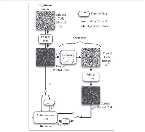
We study in this paper an authentication system which uses the fact that a printing process at very high resolution can be seen as a stochastic process due to the nature of different elements such as the paper fibers, the ink het-erogeneity, or the dot addressability of the printer. Such an authentication system has been proposed by Picard et al. [7,8] and uses 2D pseudo-random binary codes that are printed at the native resolution of the printer (2,400 dpi on a standard offset printer or 812 dpi on a digital HP Indigo printer).
The principle of the studied system in this paper is depicted in Figure 1:
• The original code is secretly exchanged between the legitimate source and the receiver.
• Once printed on a package to be authenticated, the degraded code will be scanned then thresholded by an opponent (the forger). It is important to note that at this stage thresholding is necessary for the opponent because the industrial printers can only print dots, e.g., binary versions of the scanned code.
• The opponent then produces a printed copy of the original code to manufacture his forgery.
• The receiver performs a test on an observed scanned code, being either the scanned version of the original printed code or the scanned version of the fake code. Using his knowledge on the original code, he establishes a statistical test in order to perform authentication.
One advantage of this system over previously cited ones is that it is easy to deploy since the authentication process needs only a scan of the graphical code under scrutiny and the seed used to generate the original one: no fingerprint database is required in this case.
The security of this system solely relies on the use of a PUF, i.e., the impossibility for the opponent to accurately estimate the original binary code. Different security anal-ysis have already been performed with respect to (w.r.t.) this authentication system or to very similar ones. In [9], the authors have studied the impact of multiple printed observations of same graphical codes and have shown that the power of the noise due to the printing process can be reduced in this particular setup, but not com-pletely removed due to deterministic printing artifacts. In [10], the authors use machine learning tools in order to try to infer the original code from an observation of the printed code; their study shows that the estimation accuracy can be increased without recovering perfectly the original code. In [11], the authors propose a print and scan model adapted to graphical code and derive attacks and adapted detection metrics to counter the attacks. In [12], the authors consider the security analysis in the rather similar setup of passive fingerprinting using binary fingerprints under informed attacks (the channel between the original code and the copied code is assumed to be a binary symmetric channel). They show that in this case the security increase with the code length, and they pro-pose a practical threshold when type I error (originally detected as a forgery) and type II error (forgery detected as an original) are equal.
1.2 Notations
We denote sets by calligraphic font, e.g.,X, random vari-ables (RV) ranging over these sets by the same italic capitals, e.g.,X, and their outcomes in lowercase letters, e.g.,x. EX[.] denotes the expectation overX. The cardi-nality of the setX is denoted by|X|. The sequence ofN
variables(X1,X2, ....,XN)is denotedXN.
1.3 Setup
The binary graphical code can be seen as an authentica-tion sequencexN chosen at random from the message set
XNand shared secretly with the legitimate receiver. In our authentication model,xN is published as a noisy version
yN taking values in the set of pointsVN(see Figure 1). An opponent may observeyN and, naturally, tries to retrieve the original authentication sequence. He obtains an esti-mated sequencexˆN and publish a forgery as a sequence
zN taking value in the same set of pointsVN, hoping that it will be accepted by the receiver as coming from the legitimate source. When observing a sequenceoN, which may be one of the two possible sequencesyN orzN, the
destination has to decide whether this observed sequence comes from the legitimate source or not.
The authentication model involves two channelsX → (Y,Z), and in the rest of the paper, we define the main channel as the channel between the legitimate source and the receiver, and the opponent channel as the channel between the legitimate source and the receiver but pass-ing through the counterfeiter channel (see Figure 1). The two channelsX → (Y,Z)are considered being discrete and memoryless with conditional probability distribution
PYZ|X(y,z | x). The marginal channels PY|X and PZ|X constitute the transition probability matrices of the main channel and the opponent channel, respectively.
As we shall see in the rest of the paper, authentication performances are directly impacted by the discrimina-tion between the two channels and can be maximized by channel optimization.
Note that the authentication sequencexN is generated using a secure pseudo-random number generator (PRNG) having a sufficiently large key space to prevent brute-force attacks. The seed of the PRNG can practically be transmit-ted using both a secure lossless communication channel and via a key distribution system so that the receiver can generatexN from the seed. The security of such a system is beyond the scope of this paper.
1.4 Contributions of the paper The goal of this paper is twofold:
• Firstly, it provides reliable performance
measurements of the authentication system based on a Neyman-Pearson hypothesis test (i.e., to compute accurately the probability of rejecting an authentic code and the probability of non-detecting an illegal copy, denoted as type I and type II errors,
respectively). An asymptotic expression which is more accurate than the Gaussian expression is first proposed to compute these probabilities of errors; then, the importance sampling simulation method is provided to practically estimate them. We evaluate the impact of the Gaussian approximation of the test with respect to its asymptotic expression.
• Secondly, the computation of type I and type II errors are used to derive the most favorable channels for authentication. We show first that it is in the receiver’s interest to process directly the scanned grayscale code instead of a binary version. Then, the error probabilities are used to compute for a given channel model, the configuration which maximizes the authentication performance.
formulation of these probabilities is practically confirmed by using an importance sampling method, a Monte Carlo strategy of numerical simulation that can be used to com-pute rare events. We also present how to design the chan-nel in order to maximize the authentication performance for different cases of generalized Gaussian distributions and when the opponent is either passive (he undergoes the same channel as the receiver) or active (he can adapt his channel).
2 The authentication channel 2.1 Channel modeling
Let TV|X be the generic transition matrix modeling the whole physical processes used, more specifically the print-ing and scannprint-ing devices. The entries of this matrix are conditional probabilities TV|X(v | x) relating an input alphabetX and the output alphabetV. In practical and realistic situations, X is a binary alphabet standing for black (0) and white (1) elements of a digital code, and the channel output setV stands for the set of gray-level val-ues with cardinalityK (for printed and scanned images,
K = 256). Transition matrix TV|X may conceptually be any discrete distribution over the setV, but we will focus in Section 4.4 on some common and realistic distributions when analyzing numerically the performance.
The marginal distribution of the main channel PY|X is equivalent to one print and scan process, and con-sequently, we have PY|X = TV|X. On the other hand, PZ|Xdepends on the opponent processing while he has to retrieve the original sequence before reprinting it. We aim here at expressing this marginal distribution considering that the opponent tries to restore the original sequence before publishing his fraudulent sequencezN.
When performing a detection to obtain an estimated sequencexˆNof the original code, the opponent undergoes errors. These errors are evaluated with probabilitiesPe,W when confusing an original white dot with a black and
Pe,B when confusing an original black dot with a white. This distinction is due to the fact that the distribution TV|X of the physical devices is arbitrary and not neces-sarily symmetric. LetDW be the optimal decision region for decoding white dots obtained after using classical maximum likelihood decoding:
DW =v∈V : PY|X(v|X=1) >PY|X(v|X=0)
. (1)
Error probabilitiesPe,WandPe,Bare then equal to Pe,B=
v∈DW
PY|X(v|X=0), (2)
Pe,W =
v∈Dc
W
PY|X(v|X=1). (3)
whereDcWis the complementary region in the setV. The channelX → ˆXcan be modeled as a binary input binary output (BIBO) channel with transition probability matrix PXˆ|X:
PXˆ|X(xˆ=0|x=0) PXˆ|X(xˆ=1|x=0)
PXˆ|X(xˆ=0|x=1) PXˆ|X(xˆ=1|x=1)
=
1−Pe,B Pe,B Pe,W 1−Pe,W
(4)
As we can see in Figure 1, the opponent channelX →Z
is a physically degraded version of the main channel. Thus,
X → ˆX → Z forms a Markov chain with the rela-tion PXZˆ |X(xˆ,z | x) = PXˆ|X(xˆ | x)TZ/Xˆ(z | ˆx), where TZ| ˆXis the transition matrix of the counterfeiter physical device. Components of the marginal channel matrix PZ|X are
PZ|X(v|x)=
ˆ
x=0,1
PXZˆ |X(xˆ, v|x)
=
ˆ
x=0,1
PXˆ|X(xˆ|x)TZ| ˆX(v| ˆx).
(5)
Finally, we have
PZ|X(v|X=0)=(1−Pe,B)TZ| ˆX(v| ˆX=0)
+Pe,BTZ| ˆX(v| ˆX=1), (6)
PZ|X(v|X=1)=(1−Pe,W)TZ| ˆX(v| ˆX=1)
+Pe,WTZ| ˆX(v| ˆX=0). (7)
2.2 Receiver’s strategies: thresholding or not? Two strategies are possible for the receiver.
2.2.1 Binary thresholding
As a first strategy, the legitimate receiver first decode the observed sequence oN using a maximum likelihood cri-terion based on the main channel marginal distribution PY|X. He then restores a binary versionx˜N of the original messagexN using the same decision region as defined by (1) and naturally undergoes errors.
• In the opponent channel, i.e., whenON =ZN, we make use of (6) and (7) to express the corresponding error probabilities:
˜ Pe,W =
v∈Dc
W
PZ|X(v|X=1), (8)
˜
Pe,W =(1−Pe,W)
v∈Dc
W
TZ| ˆX(v| ˆX=1)
+Pe,W
v∈Dc
W
TZ| ˆX(v| ˆX=0).
˜
Pe,W =(1−Pe,W)Pe,W +Pe,W(1−Pe,B) (9) wherePe,W =
v∈Dc
W
TZ| ˆX(v| ˆX=1)andPe,B= v∈DW
TZ| ˆX
(v| ˆX=0). The same development yields
˜
Pe,B=(1−Pe,B)Pe,B+Pe,B(1−Pe,W). (10) For this first strategy, the opponent channel may be viewed as the cascade of two binary input/binary output channels:
1− ˜Pe,B P˜e,B ˜
Pe,W 1− ˜Pe,W =
1−Pe,B Pe,B Pe,W 1−Pe,W ×
1−Pe,B Pe,B Pe,W 1−Pe,W
. (11)
As we will see in the next section, in this particular case, the test to decide whether the observed decoded sequence ˜
xNcomes from the legitimate source or not is tantamount to counting the number of erroneous decoded dots.
2.2.2 Gray-level observations
In the second strategy, the receiver performs his test directly on the received sequence oN without any given decoding. We will see in Section 3.3 that this strategy is better than the previous one (see Section 3.2).
3 Impacts of the receiver’s strategies on hypothesis testing
We consider here testing whether, for a given fixed input (x1,. . ., xN), an observed independent and identically distributed (i.i.d.) sequence(o1,. . ., oN | x1,. . ., xN) is generated from a given distributionPY|X or if it comes from an alternative hypothesis associated to distribu-tionPZ|X, (oi | xi) belonging to a discrete finite set V. Practically, we are interested in performing authentica-tion after observing a sequence of N samples (oi | xi), attesting whereas this sequence comes from a legitimate source or from a counterfeiter. The receiver establishes then a decision based on a predefined statistical test and
assigns one of the two hypothesisH0orH1
correspond-ing, respectively, to each of the former cases. Accord-ing to this test, the space VN will be partitioned into two regionsH0andH1. Accepting hypothesisH0 while
it is actually a fake (the observed N sample sequence belongs toH0whileH1is true) leads to an error of type
II having probability β. Rejecting hypothesis H0 while
actually the observed sequence comes from the legiti-mate source (the observed N sample sequence belongs to H1 whileH0 is true) leads to an error of type I with
probability α. It is desirable to find a test with a min-imal probability β for a fixed or prescribed probability of type I. An optimal decision rule will be given by the Neyman-Pearson criterion. The eponymous theorem states that under the constraintα ≤ α∗, β is minimized if only if the following log-likelihood test infers the choice ofH1:
logP
N(oN |xN, H
1)
PN(oN |xN, H0) ≥γ, (12)
whereγ is a threshold verifying the constraintα≤α∗.
3.1 Authentication via binary thresholding
In the first strategy, the final observed data isx˜N and the original sequencexNis a side information containing two types of data (‘0’ and ‘1’). The conditional distribution of each random component(X˜i | xi)of the sequence (X˜N |
xN)is the same for each given type. We compute now the probabilities that describe the two random i.i.d. sequences (X˜N |xN), one per data type, and for each of the two pos-sible hypothesis. We derive then the corresponding test from (12). Under hypothesisHj,j∈ {0, 1}, these probabili-ties are expressed conditionally to the known original code
xN. LetNB = {i : xi = 0}andNW = {i : xi = 1}, with
NB= |NB|andNW = |NW|. Because of i.i.d. sequences, we have
PN(x˜N |xN, Hj)= N
i=1
P(x˜i|xi, Hj),
PN(x˜N |xN, Hj)=
i∈NB
P(x˜i|0,Hj)
×
i∈NW
P(x˜i|1,Hj).
Under hypothesisH0the channelX → ˜Xhas
distribu-tions given by (2) and (3) and we have:
PNx˜N |xN, H0
• Under hypothesisH1, the channelX→ ˜Xhas
distributions given by (9) and (10), and we have
PNx˜N |xN, H1=(P˜e,B)ne,B(1− ˜Pe,B)NB−ne,B ×(P˜e,W)ne,W(1− ˜Pe,W)NW−ne,W. Applying now the Neyman Pearson criterion (12), the test is expressed as
L1=log
PNx˜N |xN, H1
PNx˜N |xN, H0 H1 ≷
H0
γ, (13)
L1=ne,Blog
˜
Pe,B(1−Pe,B) Pe,B(1− ˜Pe,B)
+ne,Wlog
˜
Pe,W(1−Pe,W) Pe,W(1− ˜Pe,W)
H1 ≷
H0
λ1, (14)
whereλ1 = γ −NBlog
1−˜PB
1−PB
−NWlog
1−˜PW
1−PW
. This expression has the practical advantage to only count the number of errors in order to perform the authentication task but at a cost of a loss of optimality.
3.2 Authentication via gray-level observations
In the second strategy, the observed data isoN. Here again, the conditional distribution of each random component (Oi | xi)of the sequence (ON | xN)is the same for each type of data ofX. The Neyman Pearson test is expressed as
L2=log
PN(oN |xN,H
1)
PN(oN |xN,H
0)
H1 ≷
H0
λ2, (15)
which can be developed as
L2=
i∈NB
logPZ|X(oi|0)
PY|X(oi|0)
(16)
+
i∈NW
logPZ|X(oi|1)
PY|X(oi|1) H1
≷
H0
λ2,
L2=
i∈NB log
(1−Pe,W)
TZ| ˆX(oi|0)
TY|X(oi|0) +
Pe,W
TZ| ˆX(oi|1)
TY|X(oi|0)
+
i∈NW log
(1−Pe,B)
TZ| ˆX(oi|1)
TY|X(oi|1)+
Pe,B
TZ| ˆX(oi|0)
TY|X(oi|1)
H1 ≷
H0
λ2. (17)
Note that the expressions of the transition matrix mod-eling the physical processes TY|Xand TZ| ˆXare required in order to perform the optimal test.
3.3 Authentication with thresholding vs authentication without thresholding
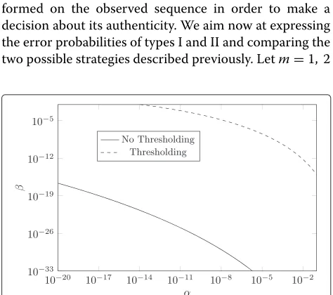
In this setup and without loss of generality, we consider only the Gaussian model with varianceσ2for the physi-cal devices TY|Xand TZ| ˆX. Figure 2 compares the receiver operating characteristic (ROC) curves associated with the two different strategies. Note that the error probabilities are computed using the results given in the next section (see Section 4.2). We can notice that the gap between the two strategies is important. This is not surprising since the binary thresholding removes information from the gray-level observation, yet this has a practical impact because one practitioner can be tempted to count the number of errors as given in (14) as an authentication score for its easy implementation. The information theo-retical analysis presented in the Appendix confirms also that authentication is more accurate without threshold-ing, and this result is in line withthe remark of Blahut in [14] where in p108 he writes that ‘information is increased if a measurement is made more precise [...] (i.e. with a refinement of the set of measurement outcomes).’
Moreover, as we will see in Section 5, the plain scan of the graphical code can be used whenever the receiver needs to estimate the opponent’s channel.
4 Toward reliable performance evaluation
In the previous section we have expressed the Neyman-Pearson test for the two proposed strategies resumed by (14) and (17). These tests may then be practically per-formed on the observed sequence in order to make a decision about its authenticity. We aim now at expressing the error probabilities of types I and II and comparing the two possible strategies described previously. Letm=1, 2
Figure 2ROC curves for the two different strategies (N=2, 000,
be the index denoting the strategy; a straightforward cal-culation gives
αm= l>λm
PLm(l|H0), (18)
βm=
l<λm
PLm(l|H1). (19)
wherePLm(l| Hj)is the distribution of the log-likelihood ratioLmunder hypothesisHj.
4.1 Gaussian approximation
As the lengthNof the sequence is generally large, we use the central limit theorem to study the distributionsPLm, m=1, 2 (a similar strategy was proposed in [15]).
• For the binary thresholding strategy,ne,Wandne,Bin (14) are binomial random variables depending on the origin of the observed sequence. LetNxstand for the
number of data of typexin the original code andPe,x
the cross-over probabilities emerging from typexin the BIBO channels (4) or (11). WhenNis large enough, the binomial random variables can be approximated with a Gaussian distribution. We have
ne,x∼N(NxPe,x, NxPe,x(1−Pe,x)). (20)
From (14),L1is a weighted sum of Gaussian random
variables and one can obviously deduce the
parameters of the normal approximation describing the log-likelihoodL1.
• For the second strategy, i.e., when the receiver tests directly the observed gray-level sequence, the log-likelihoodL2in Equation 17 may be expressed as
two sums of i.i.d. and becomes
L2=
i∈NB
(oi, 0)+
i∈NW (oi, 1)
H1 ≷
H0
λ2, (21)
where(v, x)is a function: X×V →Rhaving some distribution with mean and variance equal to
mx=E[(V, x)|Hj]=
v∈V
(v, x)P(v|x,Hj),
(22)
and
var[(V,x)|Hj]=
v∈V
((v,x)−mx)2P(v|x,Hj),
(23)
withP=PY|X(respectivelyP=PZ|X) forj=0
(respectively 1). The central limit theorem is then used again to approximate the distribution ofL2and
compute type I and type II error probabilities.
4.2 Asymptotic expression
In this section, we drop the subscribe m denoting the strategy as all the subsequent analysis is common for both of them. One important problem is the fact that the Gaus-sian approximation proposed previously provides inaccu-rate error probability values when the thresholdλin (18) and (19) is far from the mean of the log-likelihood random variableL. Chernoff bound and large deviation theory [16] are preferred in this context as very small error probabil-ities of types I and II may be desired [17]. Given a real numbers, the Chernoff bound on type I and type II errors may be expressed as
α=Pr(L≥λ|H0)≤e−sλgL(s;H0)for anys>0,
(24)
β=Pr(L≤λ|H1)≤e−sλgL(s;H1)for anys<0,
(25)
where the function gL(s;Hj) , j = 0, 1 is the moment generating function of the random variableLdefined as
gL(s;Hj)=EPL(L|Hj)
esL. (26)
where expectation is performed with respect to distribu-tionPL(L|Hj). Reminding thatLis a sum ofN indepen-dent random variables, asymptotic analysis in probability theory (whenNis large enough) shows that bounds simi-lar to (24) and (25) are much more appropriate for estimat-ingα andβ than the Gaussian approximation especially whenλis far fromE[L], namely when bounding the tails of a distribution [16,17]. The tightest bound is obtained by finding the value ofsthat provides the minimum of the right-hand side (RHS) of (24) and (25), i.e., the minimum ofe−sλg
L(s; Hj) for eachj = 0, 1. Taking the derivative, the values that provides the tightest bound under each hypothesis is such thata
λ=
dgL(s;Hj)
ds
gL(s; Hj)
s=˜sj = d
dslngL(s;Hj)
s=˜sj
. (27)
We introduce the semi-invariant moment generating function after an acute observation of the identity (27). The semi-invariant moment generating function ofLis
μL(s;Hj)=lngL(s; Hj). (28)
This function has many interesting properties that ease the extraction of an asymptotic expression for (24) and (25) [17]. For instance, this function is additive for the sum of independent random variables, and we have
μL(s;Hj)=
i∈NB
μi, 0(s;Hj)+
i∈NW
μi, 1(s;Hj), (29)
observed sequence comes from the distribution associ-ated to hypothesis Hj. In addition, relation (27) may be expressed as the sum of the derivatives at the value ˜sj optimizing the bound:
λ=
i∈NB
μi, 0(˜sj;Hj)+
i∈NW
μi, 1(˜sj; Hj). (30)
Chernoff bounds on type I and type II errors (24) and (25) may then be expressed as
α=Pr(L≥λ|H0)
≤ exp ⎡ ⎣
i∈NB
μi, 0(˜s0;H0)− ˜s0μi, 0(˜s0;H0) (31)
+
i∈NW
μi, 1(˜s0;H0)− ˜s0μi, 1(˜s0;H0)
⎤⎦ ,
and
β=Pr(L≤λ|H1)
≤ exp ⎡ ⎣
i∈NB
μi, 0(s˜1; H1)− ˜s1μi, 0(˜s1;H1)
(32)
+
i∈NW
μi, 1(˜s1;H1)− ˜s1μi, 1(˜s1;H1)
⎤ ⎦ .
The distribution of each random component(Oi|xi)in the sequence (ON |xN)is the same for each type of dataX, and consequently,μi,x(s;Hj)=μx(s;Hj), i.e.,μi,x(s;Hj) is independent fromifor each type of datax. The RHS in (31) and (32) can be simplified as
expNB
μ0(˜sj;Hj)− ˜sjμ0(˜sj;Hj)
+NW
μ1(˜sj;Hj) − ˜sjμ1(˜sj;Hj)
.
(33)
Roughly speaking, Cramér’s theorem [16] states that for sufficiently largeN, the upper bounds expressed forj =
0, 1 in (33) are also lower bounds forαandβ, respectively. Thus, one can write forNB≈NW ≈N/2 :
lim N→∞
2
Nlnα=
μ(˜s0;H0)− ˜s0μ(s˜0; H0)
, (34)
lim N→∞
2
N lnβ=
μ(˜s1;H1)− ˜s1μ(s˜1; H1)
, (35)
wheres˜0>0,˜s1< 0,μ(˜sj;Hj)= μ0(˜sj;Hj)+μ1(s˜j; Hj),
μ(s˜j; Hj) = μ0(˜sj;Hj)+μ1(˜sj;Hj). A modified asymp-totic expression including a correction factor is
evalu-ated for the sum of an i.i.d random sequence (see [17], Appendix 5A), and for largeN, we have
α =Pr(L≥λ|H0),
→ N→∞
1 ˜
s0√Nπ μ(˜s0;H0)
expN2 μ(s˜0;H0)−˜s0μ(˜s0;H0)
.
(36)
and
β =Pr(L≤λ|H1),
→ N→∞
1
|˜s1|√Nπ μ(˜s1;H1)exp
N
2
μ(˜s1;H1)−˜s1μ(˜s1;H1)
,
(37)
where μ(s˜j; Hj) = μ0(˜sj;Hj) + μ1(s˜j; Hj) is the sec-ond derivative of the semi-invariant moment generating function of(V,x)defined by
(v, 1)=log
(1−Pe,W)
TZ| ˆX(v|1) TY|X(v|1) +
Pe,W
TZ| ˆX(v|0) TY|X(v|1)
,
(38)
(v, 0)=log
(1−Pe,B)
TZ| ˆX(v|0)
TY|X(v|0) +
Pe,B
TZ| ˆX(v|1)
TY|X(v|0)
.
(39)
4.3 Numerical computations ofαandβvia importance sampling
This section addresses the problem of estimating numer-ically type I and type II error probabilities, i.e.,α andβ. Monte Carlo simulation method [18] gives accurate solu-tion since these probabilities can be expressed as expec-tations of a function of a random variable governed by a given probability distribution. We have
α=
vN∈H
1
PN(vN |xN,H0), (40)
=
vN∈VN
PN(vN |xN,H0)φ (vN;H1), (41)
where φ (vN;H1) = 1 whenever vN ∈ H1 and zero if
not. The probability of type I error is then expressed as the expectation ofφ (vN; H1)under distributionPN(vN |
xN,H0). In the same way, type II error probabilityβ is
the expectation ofφ (vN; H
0)under distributionPN(vN |
xN,H
1). In the sequel, we denotePN(vN |xN, H0)=PNY|X
andPN(vN |xN,H
1)=PNZ|X, and we have
α=EPN Y|X
φ (VN;H1)
, (42)
β=EPN Z|X
φ (VN;H0). (43)
Monte Carlo methods make use of the law of large numbers to infer an estimation forα andβ by comput-ing numerically an empirical mean for φ (vN;H1) and
each one generating an i.i.d. vectorvN, where samplesvn are driven from distributionsPY|XandPZ|X, respectively, which gives the following estimates:
ˆ
α= 1
Ntrials
Ntrials
i=1
φ ((vN)(i);H1),
(vn)(i)being generated fromPY|X
ˆ
β = 1
Ntrials
Ntrials
i=1
φ ((vN)(i);H0),
(vn)(i)being generated fromPZ|X.
The Monte Carlo estimator is unbiased (αˆ → α and ˆ
β → β) almost surely, and the rate of convergence is
Ntrials−1/2. Recalling that for a zero mean and unit variance
Gaussian random variableU,P(|U| ≤ 1.96) = 0.95, the confidence interval at 0.95 obtained from each estimation is
[αˆ− √1.96σα Ntrials
,αˆ +√1.96σα Ntrials
] (44)
[βˆ− √1.96σβ Ntrials
,βˆ+√1.96σβ Ntrials
] , (45)
whereσα (resp.σβ)is the standard deviation of the
ran-dom variable φ ((VN)(i);H1) (resp. φ ((VN)(i);H0)). As
φ ((vN)(i);H1) and φ ((vN)(i);H0) are Bernoulli random
variables with parameterαandβ, respectively, their vari-ances are easily deduced, e.g.,σα2 = α −α2 ≈ α and σβ2 = β−β2 ≈ β. Whenα andβ are very small, accu-rate estimations are then difficult to achieve with realistic number of trials. Roughly speaking, the number of trials needed isNtrials > 10
3
α (orNtrials > 10
3
β )when the desired
confidence interval at 0.95 is constrained to be about a tenth of the expected value ofαorβ. Actually, we need to evaluate numerically very small values ofαandβto draw the curveβ(α)evaluating the performance of a given test statistic. The required number of trials fails to be realistic. We propose then to use the importance sampling method [18] which enables us to generate rare events and thus reduce considerably the required number of trials. Let us consider distributionsQY|XandQZ|X over the setVsuch thatQY|XandQZ|X >0 and rewrite (42) and (43) as
EPN Y|X
φ (VN;H1)=EPN Y|X
φ (VN;H1)
QNY|X
QNY|X
,
EPN Z|X
φ (VN;H0)=EPN Z|X
φ (VN;H0)
QNZ|X
QNZ|X
.
One can then alternatively express type I and type II error probabilities by
α=EQN Y|X
φ (VN;H1)
PN Y|X
QNY|X
, (46)
β =EQN Z|X
φ (VN;H0)
PNZ|X
QNZ|X
. (47)
Monte Carlo simulation with importance sampling method gives the following two estimates:
ˆ
α= 1
Ntrials
Ntrials
i=1
φ
(vN)(i);H1
×
PNY|X((vN)(i)|xN)
QNY|X((vN)(i)|xN)
,
(vN)(i)being generated fromQNY|X, (48)
ˆ
β = 1
Ntrials
Ntrials
i=1
φ
(vN)(i); H0
×
PNZ|X((vN)(i)|xN)
QNZ|X((vN)(i)|xN)
,
(vN)(i)being generated fromQNZ|X. (49)
The problem of importance sampling is to choose an adequate functionQV|Xsuch that the variance of the esti-mated probabilities in (48) and (49) are very small. The number of trials will be considerably reduced and accurate estimations of very low values ofαandβmay be possible. Let
QY|X(s,v|x)=exp(−μx(s; H0)+s(v, x))PY|X(v|x)
and
QZ|X(s,v|x)=exp(−μx(s;H1)+s(v,x))PZ|X(v|x)
be tilted distributions over the setV , andμx(s;Hj)the semi-invariant moment generating function of(v,x) dis-tributed under hypothesisHj.
Proposition 1. The mean of the log-likelihood function (v,x)governed by the tilted distributions QY|X(s,v|x)is
μx(s;H0).
Proof.We have indeed
v∈V
(v,x)QY|X(s,v|x)=
v∈V
(v,x)exp(−μx(s;H0)+s(v,x))
×PY|X(v|x),
=
v∈V(v,x)exp(s(v,x))PY|X(v|x)
exp(μx(s;H0))
sinceμx(s;H0) = log
gx(s; H0)
, the denominator of the previous expression is simplygx(s;H0):
v∈V
(v,x)QY|X(s,v|x)=
v∈V(v,x)exp(s(v,x))PY|X(v|x)
v∈Vexp(s
(v,x))PY|X(v|x) ,
=
dgx(s;H0)
ds
gx(s;H0)
,
Finally, we have
v∈V
(v,x)QY|X(s,v|x)=μx(s;H0). (50)
The same development yields
v∈V
(v,x)QZ|X(s,v|x)=μx(s; H1). (51)
When choosing s = ˜s0 forQY|X(s,v | x) and s = ˜s1
forQZ|X(s,v|x), the mean of the log-likelihood function
(v,x)governed by these tilted distributions will be equal to the thresholdλof the test 30.
Proposition 2. The variances of the estimations in (48) and (49) go to zero as the number of dots is sufficiently large.
Proof. To show this, let oN be the observed samples coming from the main channel, e.g., driven from the tilted distributionQNY|X(˜s0,vN|xN). We have
QNY|X(˜s0,oN|xN)=exp
⎛ ⎝−
i∈NB
μi, 0(˜s0;H0)−
i∈NW
μi, 1(˜s0;H0)
+ ˜s0
i∈NB
(oi, 0)+ ˜s0
i∈NW (oi, 1)
⎞ ⎠
×PNY|X(oN |xN).
Recalling that μ(s˜j; Hj) = μ0(˜sj;Hj) +μ1(˜sj;Hj), for
NB≈NW≈N/2, we have
QNY|X(˜s0, oN |xN)=exp
⎛ ⎝−N
2μ(˜s0;H0)+ ˜s0 ⎛ ⎝
i∈NB (oi, 0)
+
i∈NW (oi, 1)
⎞ ⎠ ⎞
⎠PNY|X(oN |xN).
By the law of large numbers, the sum of N/2 log-likelihood functions of the observed samples(oi |x)
gov-erned by the tilted distribution, converges in probability to its mean value asNis sufficiently large:
i∈NB (oi, 0)
P
→ N
2
v∈V
(v, 0)QY|X(˜s0,v|0)=
N
2μ
0(˜s0;H0),
i∈NW (oi, 1)
P
→ N
2
v∈V
(v, 1)QY|X(˜s0,v|1)=
N
2μ
1(˜s0;H0).
Recalling thatμ(˜sj;Hj) = μ0(˜sj;Hj)+μ1(˜sj;Hj), and from proposition 1, we have
⎛ ⎝
i∈NB
(oi, 0)+
i∈NW (oi, 1)
⎞ ⎠ P
→ N
2μ
(s˜ 0;H0).
Equivalently, when observed samples come from the opponent channel, e.g., drawn from the tilted distribution
QNZ|X(˜s1, vN |xN), we have
⎛ ⎝
i∈NB
(oi, 0)+
i∈NW (oi, 1)
⎞ ⎠ P
→ N
2μ
(˜s 1;H1).
Finally, we have
QNY|X(s˜0,oN|xN)
P →exp −N 2
μ(˜s0;H0)−˜s0μ(s˜0;H0)
×PYN|X(oN |xN) (52)
and
QNZ|X(˜s1, oN|xN)
P →exp −N 2
μ(˜s1; H1)−˜s1μ(˜s1;H1)
×PZN|X(oN |xN). (53)
The variance ofφ (VN;H1)
PN Y|X QNY|X
whenVN is governed
by the tilted distribution QNY|X(˜s0, vN | xN) is then (the
functionφ (.)being 0 or 1)
varQN Y|X
φ(VN;H1) PNY|X
QNY|X
=EQN Y|X
⎡
⎣φ2(VN;H1)
PYN|X
QNY|X 2⎤
⎦−α2,
=EPN Y|X
φ(VN;H1)
PNY|X
QNY|X
−α2,
P →EPN
Y|X
φ(VN;H1)
1
exp−N2 (μ(˜s0;H0)−˜s0μ(˜s0;H0))
−α2.
The denominator in the expectation, i.e., exp−N2
μ(˜s0;H0)− ˜s0μ(˜s0; H0)
Cramér-Chernoff bound proposed in (34). We then have
varQN Y|X
φ (VN;H1)
PYN|X
QNY|X
P →αEPN
Y|X
φ (VN;H1)
−α2.
Finally, sinceEPN Y|X
φ (VN;H1)
= α (42), the variance goes to zero asNis large enough:
varQN Y|X
φ (VN;H1)
PNY|X
QNY|X
P →0.
The same development gives
varQN Z|X
φ (VN;H0)
PNZ|X
QNZ|X
P →0.
4.4 Practical performance analysis
Without loss of generality, we use in our analysis a gener-alized Gaussian distribution to model the physical device, i.e., the association of a printer with a scanner, used by the legitimate sourceTY|X(v|x)and by the counterfeiter
TZ| ˆX(v| ˆx):
p(v|x)= b 2a(1/b)e
−(|v−m(x)|/a)b
, (54)
where m(x) is the mean and the parameter a can be computed from the varianceσ2=var[V]:
a=σ (1/b)/ (3/b). (55)
The parameterb is used to control the sparsity of the distribution, for example, whenb = 1 the distribution is Laplacian,b = 2 the distribution is Gaussian, andb → +∞the distribution is uniform. The resulting distribution is first discretized then truncated to provide values within [ 0,. . ., 255] to model a scanning process. Each channel is parametrized in this case by four parameters, two per each type of dots, mb = m(0) and σb for black dots andmw = m(1) andσwfor white dots. Note that other print and scan models that take into account the gamma transfer function or additive noise with input dependent variance can be found in [19], but the general methodol-ogy of this paper is not dependent on the model and can still be applied.
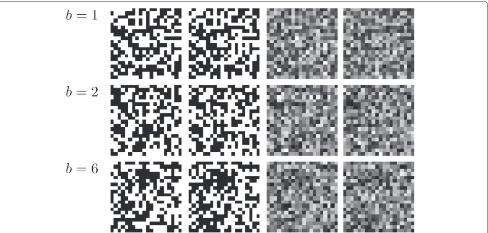
Figure 3 illustrates the different effects of the general-ized Gaussian distributions on the main and the opponent channels of same mean and variance andb=1 (Laplacian distribution),b = 2 (Gaussian distribution), andb = 6, i.e., close to a uniform distribution.
In order to assess the accuracy of the computations of αandβusing either the Gaussian approximation given by (18) and (19), the asymptotic expression given by (36) and (37), or the Monte Carlo simulations using importance
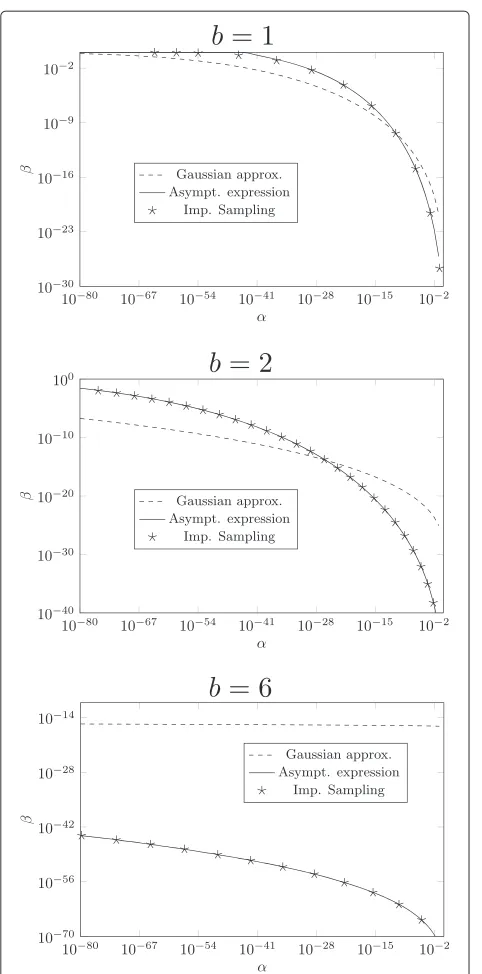
sampling given by (48) and (49), we derive ROC curves for generalized Gaussian distributions andb= {1, 2, 6}.
Figure 4 illustrates the gap between the estimation ofα andβusing the Gaussian approximation and the asymp-totic expression or the Monte Carlo simulations. The Monte Carlo simulations confirm the fact that the derived Cramér Chernoff bounds are tight, and the difference between the results obtained with the Gaussian approxi-mation are very important especially for close to uniform channels. We can also notice that for the same channel power, the authentication performances are better forb=
6 then forb=2 andb=1.
5 Optimal configurations for authentication
The goal of this section is to derive configurations that are optimal regarding authentication, i.e., to derive configura-tions that for a givenαminimizeβ.
5.1 Optimal configurations by modification of the printing channel
5.1.1 Problem setting
This authentication problem can be seen as a game where the main goal of the receiver, for a given false alarm proba-bilityα, is to find a channel that minimizes the probability of missed detection β. Practically, this means that the channel can be chosen by using a given quality of paper, a different ink, and/or by adopting an appropriate res-olution. For example, if the legitimate source wants to decrease the noise variance, he can choose to use over-sampling to replicate the dots; on the contrary, if the legitimate source wants to increase the noise variance, he can use a paper of lesser quality. It is important to recall that because the opponent will have to print a binary ver-sion of its observation, and because a printing device at this very high resolution can only print binary images, the opponent will in any case have to print with decoding errors after estimationXˆ.
We analyze two scenarios described below:
• The legitimate source and the opponent have identical printing devices; practically, this means that they use exactly the same printing setup. In this case, the legitimate source will try to look for the channelC such that for a givenα, the legitimate party will have a probability of missed detectionβ∗such that
β∗=min
C β(α). (56)
In this case, the opponent is passive and has no strategy but duplicating the graphical code.
• The opponent can modify its printing channelCo
Figure 3Example of a 20×20 code which is printed and scanned by an opponent.Main and opponent channels are identical,mb=50, mw=150,σb=40, andσw=40.
being detected. The opponent then tries to maximize the probability of false detection by choosing the adequate printing channel, and the legitimate sources will adopt the printing channelClwhich will
minimize the probability of false detection. We end up with what is called a min-max game in game theory, where the optimalβ∗is the solution of
β∗=min
Cl max
Co
β(α). (57)
In this case, the opponent is active since he tries to adapt his strategy in order to degrade the
authentication performance.
Because the expressions ofβ(α)is not simple and have to be computed using the asymptotic expressions (31) and (32), we cannot solve this problem analytically and we have to use numerical calculus instead.
We conduct this analysis for the generalized Gaussian model, where we assume that the parameters mb and
mware constant for the main and the opponent channels (which implies that the scanning process has the same calibration for the two types of images). We assume that the main channel and the opponent channel variances are respectively denotedσm2 andσo2and are identical for black and white dots.
5.1.2 Passive opponent
Here, the opponent has to undergo a channel identical to the main channel; the only parameter of the
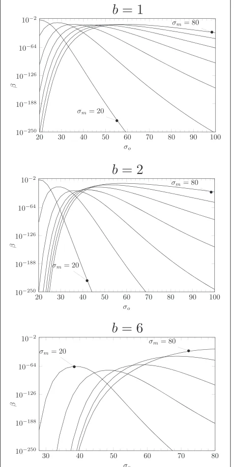
optimiza-tion problem (56) is consequentlyσm. Figure 5 presents the evolution ofβ w.r.t.σm forα = 10−6andmb = 50,
mw=150. For each channel configuration, we can find an optimal configuration; this configuration offers a smaller probability of error forb = 6 than forb = 2 orb = 1. It is not surprising to notice that in each case,βis impor-tant wheneverσm is very small (i.e., when the print and scan noise is very small, hence the estimation of the origi-nal code is easy) or very large (i.e., when the print and scan noise is so important that the original and forgery become equally noisy).
5.1.3 Active opponent
In this setup, the opponent can use a channel of differ-ent variance σo2 than the main channelσm2 and tries to solve the game defined in (57). Figure 6 shows the evo-lutions ofβ w.r.t.σo for differentσm. We can see that in each case it is in the opponent interest to optimize his channel. Note that even if we assume that the opponent print and scan channel is perfect (xˆN = zN), because the input of the printer has to be binary and because the opponent will make decoding errors by estimating the original code, the copied printed code will be necessar-ily different from the original printed code (see Figure 1), which implies a perfect discrimination between the two hypotheses.
Figure 7 shows the evolution of best opponent strategy max
σo
βw.r.t.σm. By comparing it with Figure 5, we can see
Figure 4Comparison between the Gaussian approximation, the asymptotic expression, and Monte Carlo simulations forb=1, b=2, andb=6.Main and opponent channels are identical, mb=50,mw=150,σb=40, andσw=40.
6 Impact of the estimation of the print and scan channel
The previous scenarios assume that the receiver has a full knowledge of the print and scan channel. Here, we assume that the receiver also has to estimate the opponent chan-nel before performing authentication. From the estimated parameters, the receiver will compute a threshold and a
Figure 5Evolution ofβw.r.t.σm(α=10−6).Main and opponent
channels are identical,mb=50 andmw=150.
log-likelihood test. Depending on the number of observa-tionsNo, the estimated model and test will decrease the performance of the authentication system.
Figure 6Evolution of the probability of non-detectionβw.r.t.σo for differentσm.The plots arriving from left to right showσm varying from 20 to 80 with an increment of 10.mb=50,mw=150, andα=10−6.
distributions are discrete and have the finite support of the gray-level range.
Figure 8 shows the authentication performances using an estimated Gaussian model (b = 2)fromNo = 2, 000 observed symbols. We can notice that the performance is very close to an exact knowledge of the model. This analysis shows also that if the receiver has some assump-tions of the opponent channel and enough observaassump-tions,
Figure 7Evolution of best opponent strategy max σo
βw.r.t.σm.
mb=50,mw=150, andα=10−6.
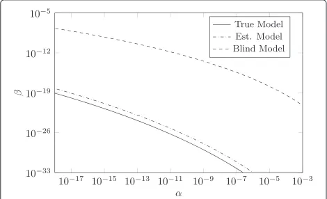
he should perform model estimation instead of using the thresholding strategy. Figure 9 shows the importance of model estimation when comparing it to a blind authen-tication test when the receiver assumes that both the opponent channel and his channel are identical.
7 Conclusions
Figure 8Authentication performance using model estimation with the EM algorithm (N=2, 000,No=2, 000,σ=52, mb=50,andmw=150).The asymptotic expression is used to
derive the error probabilities.
• The nature of the receiver’s input is of upmost importance, and thresholding is a bad strategy with respect to getting an accurate version of the genuine or forged code, except if the system requires it, due for example to computational requirements. • The Gaussian approximation used to compute the
ROC of the authentication system are not valuable anymore for very low type I or type II errors. Cramér Chernoff bound or Monte Carlo simulations using importance sampling can be used instead to achieve accurate values of these probabilities. The proposed methodology is not impacted by the nature of the noise and can be applied for different memoryless channels that are more realistic for modeling the printing process.
Figure 9Importance of model estimation when compared to a blind authentication test.ROC curves comparing different degrees of knowledge about the opponent channel while the true opponent printing process model has parameters (σ =40,mb=40, and μw=160). ‘True model’: the receiver knows exactly this model, ‘Blind model’: the receiver uses arbitrarily his printing process to model it, and ‘Est. model’: the receiver estimates the opponent channel using No=2, 000 observations.
• It is in the opponent’s interest to adapt its channel in order to decrease the authentication performances of the system; this can be possible by solving a max-min game.
• If the opponent’s print and scan channel remains unknown for the receiver, he can use estimation techniques such as the EM algorithm in order to estimate the channel.
Our future works will consist in evaluating the impact of the noise model on the authentication performance; this first analysis suggests that sparse distributions are less favorable for authentication than dense distributions, but this has to be confirmed by a deeper study.
Endnote
aOne can show thate−sλg
L(s;Hj)is a convex function ofs.
Appendix
Information theoretic comparison between hypothesis testing with and without thresholding
In this appendix, we aim at establishing an inequality between the average of the two log-likelihood tests (14) and (15). The greater is the discrimination between the two distributions involved in the log-likelihood test, the best is the authentication performance. The expected value of the log-likelihood test (12) with respect to any of the two distributions involved in the ratio is the Kullback-Leibler divergence ordiscriminationdefined as
L(PNY|X;PNZ|X)=
vN∈VN
PNY|X(vN |xN)logP N
Y|X(vN |xN)
PNZ|X(vN |xN),
(58)
the base of the logarithm being arbitrary. In the remainder of this paper, we settle on base 2.
In ([14], p. 114), the author provides an interesting inequality relating the discrimination to type I and type II errors in hypothesis testing. This relation is stated by the following lemma:
Lemma 1. (see the former reference for the proof ) For any partition(H0, H1) of the observation spaceVN, the
probabilities of type I and II errors satisfy
L(PNY|X;PNZ|X)≥αlog α
1−β +(1−α)log 1−α
β . (59)
discrimina-tion quantity for the two proposed strategies in order to establish the desired inequality:
L(PN(X˜N |xN,H0); PN(X˜N |xN,H1))
=
˜
x1 · · ·
˜
xN
PNx˜N |xN, H0
logP
Nx˜N |xN, H
0
PNx˜N |xN, H1,
(60)
and
L(PN(ON |xN,H0); PN(ON |xN,H1))
=
v1 · · ·
vN
PNY|X(vN |xN)logP N
Y|X(vN |xN)
PZN|X(vN |xN). (61)
For the sake of simplicity, we develop proofs and details for the second strategy only and give results for the thresh-olding case for which all developments are likewise the former. Regarding the additivity theorem ([14], theorem 4.3.7) for independent sequences and reminding that the distribution of each component of the sequence (ON |xN) is the same for each type of data x, the discrimination quantity becomes
L(PN(ON |xN,H0); PN(ON |xN,H1))
=NW×
v∈V
PY|X(v|1)log
PY|X(v|1)
PZ|X(v|1)
+NB×
v∈V
PY|X(v|0)log
PY|X(v|0)
PZ|X(v|0) .
(62)
Given a composition (or relative frequency) forX PX = {NW/N, NB/N}, we have
L(PN(ON |XN,H0); PN(ON|XN,H1))
=N×L(PY|X; PZ|X |PX),
(63)
whereL(PY/X; PZ/X | PX)is the average discrimination. Similarly, we obtain for the first strategy the relation
L(PN(X˜N|XN,H0);PN(X˜N|XN,H1))=N×L(Pe,x;P˜e,x|PX). (64)
Corollary 1. Given an i.i.d outcome XN =xN with com-position, or type PX, for any partition of the observation
space (H0, H1), the probabilities of type I and II errors
satisfy
L(PY|X;PZ|X|PX)≥ 1
N
αlog α
1−β+(1−α)log 1−α
β
.
(65)
Proof. The proof is straightforward by combining (59) and (63).
Corollary 2. Consider a partition of the observation space (H0, H1) with probability of type I error α; then, the
probability of type II error is lower bounded by
β≥2−[NL(PY|X;PZ|X|PX)+h(α)]/(1−α). (66)
Proof. From the previous corollary, we have
−(1−α)logβ≤NL(PY|X; PZ|X|PX)−αlogα −(1−α)log(1−α)+αlog(1−β).
Settingh(α)= −αlogα−(1−α)log(1−α), which is the binary entropy (≤1), and observing thatαlog(1−β)≤0, we can write the inequality
−(1−α)logβ≤NL(PY|X; PZ|X|PX)+h(α). (67)
It is desired that this lower bound is very small which is obviously possible with large values of the quantity
L(PY|X; PZ|X |PX).
Theorem 1. For the two strategies of the receiver, we have L(PY|X; PZ|X |PX)≥L(Pe,x; P˜e,x|PX)