Volume 2008, Article ID 256896,16pages doi:10.1155/2008/256896
Research Article
Iterative Object Localization Algorithm Using Visual Images
with a Reference Coordinate
Kyoung-Su Park,1Jinseok Lee,1Milutin Stana´cevi´c,1Sangjin Hong,1and We-Duke Cho2
1Mobile Systems Design Laboratory, Department of Electrical and Computer Engineering, Stony Brook University, Stony Brook, NY 11794, USA
2Department of Electronics Engineering, College of Information Technology, Ajou University, Suwon 443-749, South Korea
Correspondence should be addressed to We-Duke Cho,[email protected]
Received 29 July 2007; Revised 11 March 2008; Accepted 4 July 2008 Recommended by Carlo Regazzoni
We present a simplified algorithm for localizing an object using multiple visual images that are obtained from widely used digital imaging devices. We use a parallel projection model which supports both zooming and panning of the imaging devices. Our proposed algorithm is based on a virtual viewable plane for creating a relationship between an object position and a reference coordinate. The reference point is obtained from a rough estimate which may be obtained from the preestimation process. The algorithm minimizes localization error through the iterative process with relatively low-computational complexity. In addition, nonlinearity distortion of the digital image devices is compensated during the iterative process. Finally, the performances of several scenarios are evaluated and analyzed in both indoor and outdoor environments.
Copyright © 2008 Kyoung-Su Park et al. This is an open access article distributed under the Creative Commons Attribution License, which permits unrestricted use, distribution, and reproduction in any medium, provided the original work is properly cited.
1. INTRODUCTION
The object localization is one of the key operations in many tracking applications such as surveillance, monitoring and tracking [1–8].In these tracking systems, the accuracy of the object localization is very critical and poses a considerable challenge. Most of localization methods use geometric relationship between the object and sensors. Acoustic sensors have been widely used in many localization applications due to their flexibility, low cost, and easy deployment. The acoustic sensor provides directional information in angle of the source with respect to the sensor coordinates which are used to create a geometry for localization. However, an acoustic sensor is extremely sensitive to its surrounding environment with noisy data and does not fully satisfy the requirement of consistent data [9]. Thus as a reliable tracking method, visual sensors are often used for tracking and monitoring systems as well [10,11]. The visual localization has a potential to yield noninvasive, accurate, and low-cost solution [12–14].
Multiple-image-based multiple-object detection and tracking are used in indoor and outdoor surveillance, and give a delicate and complete history of an interested object’s
action [2, 15, 16]. The object tracking can be simply
concerned into a 2D tracking problem on the ground plane [2,17–19]. The establishment of correspondences in multiple images can be achieved by using a field of view lines [2,20]. Besides, for the selection of the best view about interested objects, a camera movement such as zooming and panning is required [19].
There are many localization methods which use image sensors [5,6,13,21–25]. Most of conventional localization methods follow two steps of operation. Initially, the camera
parameters are computed offline using known objects or
pattern images. Then using additional information such as control points in the scene or techniques such as structure from motion, the relative displacements of a camera are estimated [21, 26]. Basically, these studies can sufficiently
localize objects from 3D reconstruction. Once the sufficient
number of points is observed in multiple images from different positions, it is mathematically possible to deduce the locations of the points as well as the positions of the
original cameras, up to a known factor of scale [21]. In
However, in many applications, it is not easy to obtain calibration patterns [29,30]. In order to alleviate the effect of the calibration patterns, some methods based on self-calibration use the point matching from image sequences
[29–34]. In these methods, the image feature extraction
should be very accurate since this procedure is very sensitive to the noise [21,27,35]. Moreover, if a pair of stereo images for a single scene is not calibrated and the motions between two images are unknown, the image matching requires prohibitively high complexity [27,34–36].
The localization method based on the affine
recon-struction can be used for object localization without the concern of the complex calibration [37–40]. Basically, the relationships between physical space and geometric prop-erties of a set of cameras are considered. The method uses two uncalibrated perspective images where an image is induced by a plane to infinity [37–39,41–44]. Especially, the factorization method based on the paraperspective projection model can be used for localization [42,44,45]. In
[42], three well-known approximations such as orthography,
weak perspective and paraperspective are involved to full-perspective projection in the affine projection model. In [44, 45], shape and motion recovery is used for less complexity in depth computation. However, the localization method based on the affine structure requires at least five correspondences
in two images [37–39]. On the other hand, our proposed
method requires only one correspondence (i.e., a centroid coordinate of the detected object) in two images, where each correspondence represents the same object. Thus, the critical requirements of an effective localization algorithm in tracking applications are the computational simplicity with a simpler model where 3D reconstruction is not necessary as well as the robust adaptation of camera’s movement during tracking (i.e., zooming and panning) without requiring any additional imaging device calibration from the images. The contribution of this paper is to simplify localization method
with efficiency which does not consider 3D reconstruction
and complex calibration.
In this paper, we propose a simplified algorithm for localizing multiple objects in a multiple-camera environ-ment, where images are obtained from traditional digital
imaging devices. Figure 1illustrates the application model
where multiple people are localized in a multiple-camera environment. The cameras can freely move with zooming and panning capabilities. Within a tracking environment, the proposed method uses detected object points to find object location. We use the 2D global coordinate to represent the object location. In our localization algorithm, the distance between an object and a camera is provided by a reference point. Since the reference point is initially a rough estimate, we are motivated to obtain a more accurate reference point. Here, we use an iterative process which substitutes a previously localized position with a new reference point close to a real-object location. In addition, the proposed localization method has an advantage of using a zooming factor without being concerned about a focal length. Thus, the computational complexity is simplified in determining an object’s position which supports both zooming and panning features. In addition, the localization algorithm
Camera 1
Camera 2 A
B C
Figure1: Illustration of the model of application.
P
dp
Lc Oc
Ls
upp
Pp u
Pp
up
Viewable range Object plane
Virtual viewable plane
Actual camera plane
Figure2: Illustration of the parallel projection model.
sufficiently compensates a nonideal property such as optical
characteristics of a camera lens.
The rest of this paper is organized as follows.Section 2 briefly describes a parallel projection model with a single camera.Section 3illustrates the visual localization algorithm
in a 2D coordinate with multiple cameras. InSection 4, we
present analysis and simulation results where the localization errors are minimized by compensating for nonlinearity of the digital imaging devices. An application that uses the proposed algorithm for tracking people within a closed environment is illustrated.Section 5concludes the paper.
2. CHARACTERIZATION OF VIEWABLE IMAGES
2.1. Basic concept of a parallel projection model
In this section, we introduce a parallel projection model to simplify the visual localization, which is basically comprised of three planes: an object plane, a virtual viewable plane and
an actual camera plane. InFigure 2, an objectP placed on
an object plane is projected to both a virtual viewable plane
and an actual camera plane, and Pp denotes the projected
object point on the virtual viewable plane. The distance
P
dp1
Lc1
Oc
Ls
upp1 Ppp1 u
Ppp1 up1
Viewable range
Object plane 1
Virtual viewable plane 1 Actual camera
plane 1 (a) Small zooming factor (z1)
P
dp2
Lc2 Oc
Ls
upp2 Ppp2
u
Ppp2 up2
Viewable range
Object plane 2
Virtual viewable plane 2 Actual camera
plane 2
(b) Large zooming factor (z2)
Figure3: Illustration of the model of zooming in terms of two different zooming factors.
and an object plane. up and up p denote the position of
projected object Pp on both the actual camera plane and
the virtual viewable plane. The virtual viewable plane is in parallel with the object plane by distancedp.LcandLsdenote each length of the virtual viewable plane and the actual camera plane, respectively. The virtual viewable plane is for
the connection between the positionP on the object plane
and the position Pp on the actual camera plane; it has an
advantage of simplifying the computation process.
Since the size of image sensor is much smaller than the virtual viewable plane, the viewable range starts from a point
Oc. Thus the camera model of parallel projection model is
similar to a pin-hole camera. All planes are represented as
u- andv-axes but we useu-axis for the explanation of the parallel projection model in this section. SinceOcrepresents the origin of both the virtual viewable plane and the camera plane, two planes are placed on the same camera position.
However, inFigure 2, we drew two planes separately to show
the relationship between three planes.
In the parallel projection model, an object is projected from an object plane through a virtual viewable plane to an actual camera plane. Hence, as formulated in (1),up p is expressed asLc,Ls, andupthrough the proportional lines of two planes as the following:
up p=up
Lc Ls
. (1)
Thus the object P is represented from up p and the
distancedpbetween the virtual viewable plane and the object plane.
2.2. Zooming and panning
Since the size of the virtual viewable plane and the object plane are proportional to the distance between the object and the camera (dp), the length of the virtual viewable plane (Lc) is derived from the distancedpand the viewable range.
Zooming factor represents the relationship betweendp
andLc. The zooming factorzis defined as a ratio ofdpand
Lcas follows:
z= dp
Lc. (2)
Since bothdpandLcuse metric units, zooming factorz
is a constant.
Figure 3 illustrates the model of zooming in terms of
two different zooming factors. Even though the zooming
factor of a camera has changed fromz1toz2, if the distance between object and camera is not changed, the position of projected object on the virtual viewable plane is not changed. In the figure, since the distancedp1is equal to the distance
dp2, the position of the object on the virtual viewable plane is invariant but the position on the actual camera plane is variant. Thus the distance up p1 is equal to up p2 but the distanceup1is different from the distanceup2. The projected
positionsup1 andup2 on the actual camera planes 1 and 2
are expressed asup p1 =up1(Lc1/Ls) andup p2 =up2(Lc2/Ls). Sincez1=dp1/Lc1andz2=dp2/Lc2, the relationship between
up1andup2is represented asup1=up2(z2/z1).
Figure 4illustrates a special case in which two different
objects denotedP1andP2are projected to the same spot on
the actual camera plane. Pp1 andPp2 denote the projected
objects on the virtual viewable planes 1 and 2.
The objectsP1 and P2 are projected to a point on the
actual camera plane while two objects are separated as two different points on the virtual viewable plane 1 and 2. Since
the zooming factor z is equal to dp1/Lc1 and dp2/Lc2, the
relationship between the distanceup p1andup p2is expressed as up p1 = up p2(dp1/dp2). The distance up1 is equal to the
distance up2, and the distance up p1 is different from the
distance up p2. It is shown that the distance in projection
direction between an object and a camera is an important parameter for the object localization.
Now, we consider a panning factor denoted asθp that
P2
upp2 Object plane 2
P1
upp1 Object plane 1 dp1
dp2
Lc1
Lc2
Oc
Ls
Pp1
Pp2
u
up
Virtual viewable plane 2 Actual camera
plane
Pp
Virtual viewable plane 1
Figure4: Illustration of a special case in which different objects are projected to the same spot on the actual camera plane.
Camera C
θp
θc=π+θp
u
n
Camera B
θp
θc=π2+θp
u
n
Camera A
θp
θc=θp
u n
Camera D
θp
θc=32π+θp
u n
y
x
Figure5: Illustration of individual panning factors with respect to a global coordinate.
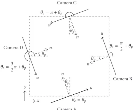
the angle difference betweenn-axis andu-axis wheren-axis represents the normal direction of the virtual viewable plane. Thus the panning angle can exist in the range of−π/2< θp< π/2. The sign ofθpis determined: the left rotation is positive and the right rotation is negative.
To get the global coordinate of the object,u-axis andv -axis in camera coordinate are translated tox-axis andy-axis in global coordinate. We define camera angle factor (θc) to represent the absolute camera angle in global coordinate. The
camera angleθc is useful to translate the object coordinate
from camera images.
Figure 5illustrates the relationship between the camera
angleθcand the panning angleθpin global coordinate. The
global coordinate is represented as x-axis and y-axis. For
example, in the position of CameraA, panning angleθp is
the angle between n- and y-axes; while in Camera D, the
panning angle is the angle betweenn-axis andx-axis. Thus
four cases of camera deployment such as CameraA,B,C,
Dhave different relationships between θcandθp. Thus the
projected objectPp(xp p,yp p) on the virtual viewable plane is derived fromxp p=xc+up pcosθcandyp p=yc+up psinθc.
Oc(xc,yc) denotes the origin on the virtual viewable plane in global coordinate.
2.3. The relationship between camera positions
and pan factors
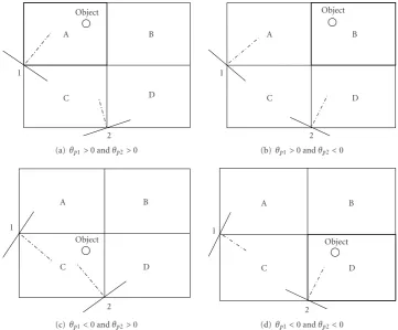
Figure 6illustrates the panning factor selection in a pair of cameras depending on an object position. Among deploy-ment of four possible cameras, such as camerasA,B,C, and
D, a pair of cameras located in adjacent axes is chosen.
In this paper, we choose camerasA and D for the
deployment of two cameras for the sake of the localization
formulation. The camera angles in Camera A and D are
expressed asθc =θp andθc = θp+ (3/2)πin terms of the
panning angleθp.
3. VISUAL LOCALIZATION ALGORITHM IN A 2-DIMENSIONAL COORDINATE
3.1. The concept of visual localization
Turning to the object localization with an estimate, consider a single-camera-based localization. In the single-camera localization, we use the estimate plane as an object plane. Figure 7illustrates the object localization using the estimate
E based on a single camera, where E denotes the estimate
which is used for a reference point. Note that the the estimate
Eas a reference point may be any position at the first time,
and it becomes close to a real position. The estimateEand
the object P are projected to two planes: virtual viewable
plane and actual camera plane. Here, the reference point
E generates the object plane. The distance de denotes the
distance between the estimate and the virtual viewable plane. In view of the projected positions, the lengthlpis obtained by the lengthlps. Hence the objectP(xp,yp) is determined from the estimateE(xe,ye).
Once we use the estimate plane as an object plane, the estimated object positionPis different from the real-object
position Pr. In other words, since any points on the ray
between the object and origin are projected to the same spot
on the actual camera plane, the real object Pr is distorted
to the point P. Thus, the localization has an error from
the distance difference of the distancesdp andde. Through the single-image sensor-based visual projection method, it is shown that an approximated localization is accomplished with a reference point.
We are now motivated to use multiple image sensors
in order to reduce the error between Pr and P. In the
case of single camera, the distance difference between the
distancesdpanddecannot be found by a single-camera view.
1
2
A B
C D
Object
(a)θp1>0 andθp2>0
1
2
A B
C D
Object
(b)θp1>0 andθp2<0
1
2
A B
C D
Object
(c)θp1<0 andθp2>0
1
2
A B
C D
Object
(d)θp1<0 andθp2<0
Figure6: Illustration of panning factor selection in a pair of cameras depending on an object position.
Pr
P E
dp
de
Lc
Oc
Ls
lp
l
Pp
Ep
lps
Object plane Object plane
Virtual viewable plane Actual camera
plane
Figure7: Illustration of the visual localization in a single camera.
be compensated by the relationship between two camera views.
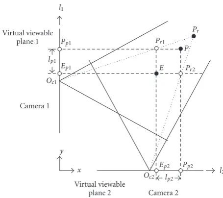
Figure 8illustrates the localization using two cameras for a simple case where both panning factors are zero, and the directions of l1- and l2-axes are aligned to y- and x-axes. Given by a reference pointE, the virtual viewable planes for
two cameras are determined. Pr1 andPr2 are the obtained
object coordinates in each single camera. In view of camera
1, the lengthlp1 between the projected pointsPp1 andEp1
supports the distance between the object plane of camera
2 and the pointP. Similarly, in the view of camera 2, the
lengthlp2between the projected pointsPp2andEp2supports
a distance between the object plane of camera 2 and the pointP. Therefore, the basic compensation algorithm is that
camera 1 compensates y-direction by the length lp1, and
camera 2 compensatesx-direction by the lengthlp1given by
a reference pointE.
Through one additional image sensor, both l1 in y
-direction and l2 in x-direction make a reference point
E(xe,ye) closer to a real-object position. HenceP(xp,yp) is
computed byxp=xe+lp2andyp= ye+lp1. Note thatPis
the localized object position through the two cameras, which still results in an error with the real-object positionPr. The
error can be reduced by obtaining a reference pointEcloser
to a real positionPr. InSection 3.5, an iterative approach is introduced for improving localization. In the next section, we formulate the multiple image sensor-based localization.
3.2. 2D localization
3.2.1. 2D localization model
Pp1 Pr1
Pr
P lp1
Ep1 E Pr2
Oc1
Ep2 Pp2 Oc2 lp2 y
x l2
l1
Camera 1
Camera 2 Virtual viewable
plane 1
Virtual viewable plane 2
Figure8: Illustration of the localization in multiple cameras.
l1 Pp1 lp1
Ep1 dp1
de1 P
l
E
dp2
de2 lp2 Pp1l2 Ep1
v1
u1
v2 u2
Virtual viewable plane 2 Virtual viewable
plane 1
Figure9: Illustration of basic localization algorithm.
is represented as P(xp,yp) in global coordinate, the 2D
localization gives a feasible solution.
To derive 2D localization equations, we use vector notation which has a benefit to express the relationship
between the estimate and the object where “” denotes a
unit vector and “→” represents a vector. For example, one
vectorris represented asAax +Bay +Caz, whereax,ay , and
az denote unit vectors towardx-, y-, andz-axes and A, B, and C are the magnitude ofx-, y-, andz-axes, respectively. Figure 9shows the basic model of object localization. The vectorsl,lp1, andlp2denote the vector from the estimateE
to the objectP, the vector from the projected estimateEp1to
the projected objectPp1on the virtual viewable plane 1, and
the vector from the projected estimateEp2 to the projected
objectPp2on the virtual viewable plane 2, respectively. The lengthslp1andlp1are the projections of the vectorlon the virtual viewable planes 1 and 2.
Figure 10 shows the projected image on the virtual
viewable planes 1 and 2 where the projected pointsPp1and
Pp2are expressed asPp1(up p1,vp p1) andPp2(up p2,vp p2) on
the virtual viewable planes 1 and 2.zp1 andzp2 denote the
z-coordinates of the projected objects in global coordinate
and are equal tozc1+vp p1andzc2+vp p2. Since the estimate
Pp1 vl
Ep1 upp1
zp1
vpp1 lp1
u1
Virtual viewable plane 1 (a)
Ep2 v2
Pp2 upp2 zp2
vpp2
lp2
u2
Virtual viewable plane 2 (b)
Figure 10: Illustration of the projected images on the virtual viewable planes 1 and 2.
has some height with the object, the projected estimate and
object have the same z-coordinate on the virtual viewable
plane 1 and 2. Thus in the figure,vp p1is different fromvp p2
whilezp1is equal tozp2. Since an estimate is a reference point, the actual estimates in the figure are not displayed on the actual camera plane. Since the projected vectorslp1andlp2
are the projection of vectorltowardl1-axis and l2-axis, the lengthslp1andlp2are equal tol·al1andl·al2.
3.2.2. Object localization based on a single camera
The projected object Pp(lp p) in l-axis is transformed into
Pp(xp p,yp p) in global coordinate. The originOc(xc,yc) is the center of virtual viewable plane. The camera deployment is expressed as the originOc(xc,yc) and camera angleθc.
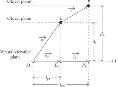
Figure 11shows the estimation with a reference point,
and a projected object. lp denotes the vector from the
origin Oc to the estimate E. The object P, estimate E,
projected objectsPp, and projected estimatesEpare denoted
viewable plane andlp =(xp−xc)ax + (yp−yc)ay in global coordinate.
The unit vectoral is represented in global coordinate
as al = cosθcax + sinθcay . The vector e is expressed as (xe−xc)ax + (ye−yc)ay . Since the lengthlpeis equal to the projection of vectoretowardl-axis (e·al), the lengthlpe is represented as:
lpe =xe−xccosθc+ye−ycsinθc. (3) Once we assume the estimate is close to the object, the lengthlp pis represented as
lp p=lps
dp
zLs
lps
de zLs
, (4)
where the lengthlps is the length of the projected estimate
and object on the actual camera plane.
InFigure 11, since the vectorlp is equal tolp pal −lpeal, the length of vectorlpis represented as follows:
lp=lp p−lpe. (5)
Since the lengthlpis the projection of the vectorltoward
l-axis (l·al), the global coordinate P(xp,yp) is related with
E(xe,ye) as follows:
xp−xecosθc1+yp−yesinθc=lp. (6) Note that since there are two unknown values of
P(xp,yp), two equations are necessary.
3.2.3. Object localization based on multiple cameras
As shown inFigure 9, once there are two available cameras
which show an object at the same time, two cameras have the following relationship:
xp−xecosθc1+yp−yesinθc1=lp1,
xp−xecosθc2+yp−yesinθc2=lp2.
(7)
The projected vector sizes of the vectorslp1 andlp2 are derived fromlp1=lp p1−lpe1andlp2=lp p2−lpe2in (5). The lengthslp p1andlp p2are represented aslp p1 lp1(de1/z1Ls1) andlp p2lp2(de2/z2Ls2) in (4). The length betweenOc1and
Pp1in an actual camera plane (lp1) and the length between
Oc2andPp2in an actual camera plane (lp2) are obtained from displayed images.
Therefore, the object positionP(xp,yp) is represented as follows:
⎡ ⎣xp
yp
⎤ ⎦=
⎡ ⎣xe
ye
⎤ ⎦+
⎡
⎣cosθc1 sinθc1
cosθc2 sinθc2
⎤ ⎦
−1⎡
⎣lp1
lp2
⎤
⎦. (8)
3.3. Effect of zooming and lens distortion
The errors caused by zooming effect and lens distortion are
the reason of scale distortion. In practice, since every general
P
l E
dp
de
e
ep lp
Oc Ep Pp
lpe
lpp
l
Object plane Object plane
Virtual viewable plane
Figure11: The estimation of a projected object.
Pr
P E
dp
de
Oc
z
Lc Ep lp Pp
z
Lc P
p
Ep lp
l
Object plane Object plane
Ideal viewable angle
Virtual viewable plane Virtual viewable
plane Actual viewable
angle
Figure 12: Illustration of actual zooming model caused by lens distortion.
camera lens has nonlinear viewable range, the zooming factor is not a constant. Moreover, since a reference point is a rough estimate, the distancedpcould be different from the distancede. However, in (4), the distancede, instead of the distancedp, is used to get the lengthlp p.
Figure 12 illustrates the actual (nonideal) zooming model caused by lens distortion where the dashed line and the solid line indicate ideal viewable angle and actual viewable angle, respectively.
For reference, zooming distortion is illustrated in Figure 13with the function of distance from the camera and various actual zooming factors measured by Canon Digital
Rebel XT with Tamron SP AF 17–50 mm Zoom Lens [46,47]
where the dashed line is the ideal zooming factor and the solid line is the actual (nonideal) zooming factor. As the distance increases, the nonlinearity property of zooming factor decreases.
To reduce the localization error, we update the lengthlp. The lengthslp pandlp pare equal tolps(Lc/Ls) andlps(Lc/Ls),
respectively. Due to the definition of zooming factor,zand
zare expressed asde/Lcanddp/Lc. Since the objectsPandPr
camera plane. Thus the actual length lp is represented as
follows:
lp=lp p
dp
de
z
z
−lpe. (9)
The distancesdeanddpare derived from
de=
xe−xpe2+ye−ype2,
dp=
xp−xp p2+yp−yp p2,
(10)
wherexpe,ype,xp p, andyp p, are equal toxc+lpecosθc,yc+
lpesinθc,xc+lp pcosθc, andyc+lp psinθc, respectively. Finally, the compensated object position P(xpr,ypr) is determined as follows:
⎡ ⎣xpr
ypr
⎤ ⎦=
⎡ ⎣xe
ye
⎤ ⎦+
⎡
⎣cosθc1 sinθc1
cosθc2 sinθc2
⎤ ⎦
−1⎡
⎢ ⎣
lp1
lp2
⎤ ⎥
⎦, (11)
where the lengthslp1andlp2are equal tolp p1(dp1/de1)(z1/z1) −lpe1andlp p2(dp2/de2)(z2/z2)−lpe1, respectively.
3.4. Effect of lens shape
The virtual viewable plane is a plane, and real camera displays a curved space. Thus, unit distances per pixel in
u- and v-axes are nonlinear on the actual camera plane.
Figure 14shows the error caused by lens shape, where the distancesdp1anddp2denote two different distances between the estimates and the camera.
Figure 15illustrate the distribution of unit distance ofu
-andv-axes on the actual camera plane. The distance between
camera and calibration sheet is 35 inches and an unit distance is 1 inch.
The translation of the distance between the estimate and the object needs the compensation for the nonlinearity by
camera calibration. In Figure 15(a), the unit distance for
u-axis is invariant in v-axis and in Figure 15(b), the unit
distance for v-axis is also invariant in u-axis. Hence in
Figure 10, the height differences of two different cameras have little effect for the overall localization error.
3.5. Iterative localization for error minimization
Once the virtual viewable plane is defined by the estimate, the localized result has the error caused by the distance difference
between the estimate E and the real object Pr. Thus the
distance between the object and the estimate is important for reducing the localization error.
The basic concept of iterative approach is to use the
previous localized positionPas a new reference pointEfor
the localization of objectPr. Thus since the reference point
E is closer to a real positionPr, the localized positionP is getting closer to a real positionPr.
Figure 16(a) illustrates the basic localization based on
two cameras where Pr represents the real object. If the
distancedp is equal to the distancede, the obtained object
0.5 1 1.5 2 2.5 3 3.5 4 The distance of object plane and
virtual viewable plane (m) 0.6
0.8 1 1.2 1.4 1.6 1.8 2 2.2 2.4 2.6
Zo
om
fa
ct
or
(
z
)
17 mm 24 mm
35 mm 50 mm
Figure 13: Illustration of zooming distortion on a function of distance from the camera and various actual zooming factors used.
Ep2
Ep1 E1
E2
Oc
Lc1
Lc2
d1
d2
Object plane Ideal viewable
range
Virtual viewable plane
Actual viewable range
Figure14: Illustration of the error caused by lens shape.
coordinate uses the coordinate ofPp1andPp2to translate the
global coordinate of the object. Thus the object point P is
closer to the real object pointPr.
Figure 16(b)shows the iterative localization. Each iter-ation gives closer object coordinate with relative computa-tional complexity. Thus the iterative approach can reduce the localization error. Furthermore, through the iteration process, the localization is becoming insensitive to the nonlinear properties.
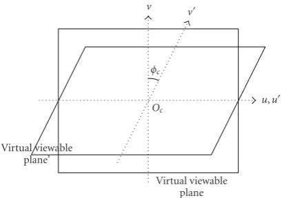
3.6. Effect of tilting angle
In surveillance system, a camera can have tilting angle to
increase viewable area. The tilting angle φc represents the
angle difference between z-axis and v-axis on the virtual
viewable plane. The tilting angle has the range as−π/2 ≤
φc< π/2.
Figure 17illustrates an example of the tilting angle where
one plane is placed on z-axis and the other has θc tilting
angle. The tilting angle φc is equal to the angle difference
u-axis
103 104 105 106 107 108
v
-axis
(a)Δu
u-axis
104 105 106 107 108
v
-axis
(b)Δv
Figure15: Illustration of unit distance distribution due to camera nonlinearity on the actual camera plane.
Sinceu-axis is invariant for the variation of tilting angle,u -axis on the virtual viewable plane is the same asu-axis on the virtual viewable plane.
The tilting angle is the reason for distortion in u
-andv-axes as shown in Figure 18.P(up,vp) and P(up,vp)
denote the project object positions of the same object within different tilting angles. The tilting angle is not affecting the
variation in u-axis. However, the tilting angle changes the
distance of the object and camera. Thus, once the distance of object and camera is changed, the zooming factor is also changed. Therefore, the tilting angle distorts the object position inu-axis.
InFigure 18, the distanceupis different from the distance
upeven if the position of camera and object is not changed.
Sinceup andup on the actual camera plane are translated
to up p andup p using the zooming factor and the distance
between the object and camera, the tilting angle is the reason for the localization error.
Figure 19illustrates the effect of tilting angle in terms of the distance between the object and the virtual viewable plane. The heightshpandhcdenote the object height and the camera height. If the camera hasφctilting angle, the distance
dpis changed by the distancedp.
In order to compensate the localization error from tilting
angle, we update the distancedptodp and then change the
l1
Pp1
lp1 Oc1 Ep1
dp1
de1 Pr1
Pr
P
Pr2 l
E
dp2
de2 lp2
l2
Pp2
Ep2 Oc2
Virtual viewable plane 2 Virtual viewable
plane 1
(a) Basic
l1
Pp1 Ep1
lp1
Oc1 dp1
Pr
P l
E
dp2 lp2 l2
Pp2
Oc2
Virtual viewable plane 2 Virtual viewable
plane 1
(b) First iteration
Figure16: Illustration of iterative localization.
v v
u,u φc
Oc
Virtual viewable plane Virtual viewable
plane’
Figure17: Illustration of an example of the tilting angle.
zooming factor for the distancedp. Thus the lengthlpin (9)
is updated as follows:
lp=lp p
d
p de
z z
−lpe, (12)
where z denotes the zooming factor when the distance
between the object and the virtual viewable plane isdp.
The distancedpis derived as follows:
dp=
up
Pp
vp
v
u
(a)φc=0
up
Pp
vp
v
u
(b)φc=10◦
Figure18: Illustration of the distortion by the tilting angle (φc).
v
n
vpp P
p
v
φc
Oc
Pp
do dp
dp
P
hp
hc
Ground
Figure19: Illustration of the effect of tilting angle.
where the distancedois computed as
do=hc−hptan−1φc. (14)
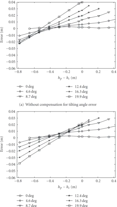
To quantify the localization error caused by tilting angle, we tested the localization error in the simple case.Figure 23 shows the setup of experiment where two cameras are placed on the left side for camera 1 and the bottom side for camera 2 in Cartesian coordinate. For simplicity, the panning factors
θp1andθp2are both zero. We denote the object is placed on
P(1.8 m, 1.8 m) andE(1.5 m, 1.5 m).
−0.8 −0.6 −0.4 −0.2 0 0.2 0.4
hp−hc(m)
−0.06
−0.05
−0.04
−0.03
−0.02
−0.01
0 0.01 0.02 0.03 0.04
Er
ro
r
(m)
0 deg 4.6 deg 8.7 deg
12.4 deg 16.3 deg 19.9 deg (a) Without compensation for tilting angle error
−0.8 −0.6 −0.4 −0.2 0 0.2 0.4
hp−hc(m)
−0.06
−0.05
−0.04
−0.03
−0.02
−0.01
0 0.01 0.02 0.03 0.04
Er
ro
r
(m)
0 deg 4.6 deg 8.7 deg
12.4 deg 16.3 deg 19.9 deg
(b) With compensation for tilting angle error (hp−hc= −0.2 m)
Figure20: Illustration of the localization error in terms of tilting angle variation.
Figure 20(a)illustrates the localization error in terms of tilting angle variation. If the tilting angle is zero, the height difference between the camera and the object (hp−hc) does not affect the localization result while the higher tilting angle makes the higher localization error. Thus the tilting angleφc
is the reason for localization error. For example, if the height of the object is 0.2 m lower than the camera height, the range of localization error is from 0.003 to 0.025 m.
Once object height is provided, the localization error is
compensated by (12). InFigure 20(b), we compensated the
localization error by denoting the camera height as 1.8 m and the object height as 1.6 m. The overall error caused by the tilting angle has the error range from 0.003 to 0.011 m. If we know the camera height and object height, the error is
compensated. Moreover, once the height difference between
−0.8 −0.6 −0.4 −0.2 0 0.2 0.4
hp−hc(m)
−0.03
−0.02
−0.01
0 0.01 0.02 0.03 0.04 0.05 0.06
Er
ro
r
(m)
1.8 (m) 2.1 (m) 2.4 (m)
2.7 (m) 3 (m) 3.3 (m) (a) Without compensation for tilting angle error
−0.8 −0.6 −0.4 −0.2 0 0.2 0.4
hp−hc(m)
−0.03
−0.02
−0.01
0 0.01 0.02 0.03 0.04 0.05 0.06
Er
ro
r
(m)
1.8 (m) 2.1 (m) 2.4 (m)
2.7 (m) 3 (m) 3.3 (m)
(b) With compensation for tilting angle error (hp−hc= −0.2 m)
Figure 21: Illustration of the localization error in terms of the distancedp(φc=12.4 deg).
error in high-tilting angle, the localization error is obviously improved. Therefore, if we expect the height of the object, the localization error can be successfully compensated.
When the height difference between the object and
cam-era is an unknown value, the compensation for localization caused by tilting angle is difficult. However, if the distance
dpis much longer than the distancedo, the tilting angle has little effect for the localization error.Figure 21illustrates the localization error in terms of the distancedpwhere the tilting
angle is 12.4 degree. When the distance dp increases, the
localization error increases but after dp is 2.7 m, the error is saturated. In the worst case, the error rate is 0.01 m error per 0.2 m height distance. For example, once the camera height difference is 6 m, the expected error is about 0.3 m. Moreover, when the camera height is 0.2 m taller than the
P lp1 E
v
u
(a) Camera 1
E lp2 P
v
u
(b) Camera 2
Figure22: Illustration of two images of camera 1 and camera 2.
object, the error range is from 0.023 to 0.04 m. Once we assume the object is placed on 0.2 m lower than the camera, the compensation reduces the error to the range of 0.006 to 0.024 m.
4. ANALYSIS AND SIMULATION
4.1. Simulation setup: basic illustration
The objective in this simulation ensures the proposed local-ization algorithm by measuring the locallocal-ization error in the real case. To show the compensation for camera nonlinearity, we chose small space which is close to the camera. In the
case of Figure 13, the distortion from camera nonlinearity
exists in 2.0 m inside space. Thus in this simulation, we use
4 m×4 m area.
Our target application is a surveillance system where most of target objects are human or vehicle. However, in this simulation, we use a small ball as a target object to simplify the target detection. There are many reasons for localization error caused by detection. For example, the centroid detection of a human is important for reducing localization error since a human is represented as a point.
If we use different positions between two camera images,
P
Camera 1
Camera 2 Viewable
range
4 m
4 m
Figure 23: Illustration of experimental setup for localizing an actual object.
1 1.5 2 2.5 3
x-axis (m) 0
0.1 0.2 0.3 0.4
Er
ro
r
(m)
Basic 1st
2nd 3rd (a)
1 1.5 2 2.5 3
y-axis (m) 0
0.1 0.2 0.3 0.4 0.5
Er
ro
r
(m)
Basic 1st
2nd 3rd (b)
Figure24: Illustration of error comparison based on the number of iterations.
Figure 22 shows the displayed images in two cameras where the lengthslp1andlp2are distances between a reference
point Eand a real-object pointP in camera 1 and camera
2, respectively. To explain the test setup, we showed the reference pointEin Figures22(a)and22(b), but actually the reference point is a virtual point.
Figure 23 shows the experiment setup to measure an actual object. In this experiment, the actual position of the object is calculated from the reference based on the parallel
projection model. InFigure 23, two cameras are placed on
0 0.5 1 1.5 2 2.5 3 3.5 0
0.5 1 1.5 2 2.5 3 3.5
(a) Trajectory performance
0 2 4 6 8 10 12
Time 0
0.5 1 1.5 2 2.5 3 3.5
x
-axis
(m)
Real Estimate
Basic First iteration (b)x-axis performance
0 2 4 6 8 10 12
Time 0
0.5 1 1.5 2 2.5 3 3.5
y
-axis
(m)
Real Estimate
Basic First iteration (c)y-axis performance
0 0.5 1 1.5 2 2.5 3 3.5 0
0.5 1 1.5 2 2.5 3 3.5
E
Real Basic
First iteration Second iteration
Figure 26: Application of the iterative localization with single estimate.
the left side for camera 1 and the bottom side for camera 2 in
Cartesian coordinate. Both camera panning factorsθp1 and
θp2are at zero.
The actual zooming factors arez1 = de1/Lc1 andz2 =
de2/Lc2, where z1 is the zooming factor when the distance
between the object plane and the virtual viewable plane
is dp1, and z2 is the zooming factor when the distance
between the object plane and the virtual viewable plane is
dp2. Now, we analyze the localization result and compare the localization error depending on the iteration process called compensation.
4.2. Localization error and object
tracking performance
Figure 24shows the error distribution of the algorithm where two cameras are positioned atOc1(1.8, 0) andOc2(0, 1.8). The actual object is located atP(1.5, 1.5). The figures illustrate the amount of localization error as a function of the reference coordinate. Since each camera has limited viewable angles, the reference coordinate located on the outside of viewable angle cannot be considered. Note that the error is minimized when the reference points are close to the actual object point. The localization error can be further reduced with multiple iterations.
The proposed localization algorithm is also used for a tracking example. In this example, an object moves within a
4 m×4 m area, and the images are obtained from the real
cameras. We first applied the proposed noniterative local-ization algorithm with compensation in tracking problems. Each time the object changes coordinates, its corresponding estimation is generated.Figure 25(a)illustrates the trajectory result of localization. After the compensation, the tracking
performance is improved. Figures25(b)and25(c)illustrate
the tracking performance in thex-axis and they-axis. These
(a) Snapshot 1
(b) Snapshot 2
Figure27: The snapshots of the tracking environment with moving camera based on the proposed localization algorithm. Human face is used to localize a person. The circle represents the actual coordinate of the person within the room.
figures clearly show that the compensation improves the tracking performance but the localization error still exists.
Similarly, the proposed iterative localization algorithm is used in the same tracking example. In this case, only one reference coordinate is used for the entire localization. The chosen estimate is outside the trajectory as shown in Figure 26. This figure illustrates the trajectory result of localization. There is a significant error with the one iteration since the estimated coordinate is not close to the object. Note that the error increases if the object is further away from the estimated coordinate. However, successive iterations eliminated the localization error as shown in the figure.
4.3. Application of the algorithms
(a) Frame1 in Camera1
(b) Frame2 in Camera1
(c) Frame3 in Camera1
(d) Frame4 in Camera1
(e) Frame5 in Camera1
(f) Frame1 in Camera2
(g) Frame2 in Camera2
(h) Frame3 in Camera2
(i) Frame4 in Camera2
(j) Frame5 in Camera2 Figure28: Illustration of detection results for people localization in an outdoor environment.
0 2 4 6 8 10 12 14 16
0 2 4 6 8 10 12 14 16 18 20
3◦ 34
◦
Person A (actual) Person A (computed)
Person B (actual) Person B (computed)
Camera 1 Camera 2
Figure 29: Illustration of two objects trajectory in an outdoor environment.
coordinates of the center of the room is chosen as the initial reference coordinate. The cameras follow the object during the localization. When the object is detected by individual camera, the coordinate of the camera images are combined for actual coordinate. The actual coordinate is shown in the tracking environment. In the experiment, cameras are following the object through panning.
Figure 28 illustrates object detection in outdoor envi-ronment where two objects are used for evaluating the proposed localization algorithm. Both cameras are placed on the same side and the panning angles for camera 1 and camera 2 are 3◦ and 34◦, respectively. Figure 29illustrates two objects trajectories in an outdoor environment. Since the method is computationally simple, the total computation time is proportional to the the number of objects, which is not a significant with respect to overall computation. As shown in the figure, the trajectory computation errors are negligibly small for the practical use. The average error in terms of the distance between the actual trajectories and the computed trajectories is 0.294 m and 0.296 m for
personsAandB, respectively. However, the maximum error
can go up to as much as 0.608 m (3%) for person B. In addition to the localization algorithm computation errors, note that additional contributing factors on the errors are the measurements of the distances between the cameras and persons, and the selected center point of the detected regions of the persons used in the computation.
5. CONCLUSION
This paper proposes an accurate and effective object localiza-tion algorithm with visual images from unreliable estimate coordinates. In order to simplify the modeling of visual localization, the parallel projection model is presented where simple geometry is used in computation. The algorithm minimizes the localization error through iterative approach with relatively low-computational complexity. Nonlinearity distortion of the digital image devices is compensated during
the iterative approach. The effectiveness of the proposed
algorithm in object position localization as well as tracking is illustrated. The proposed algorithm can be effectively applied in many tracking applications where visual imaging devices are used.
ACKNOWLEDGMENTS
This research is supported by Foundation of Ubiquitous Computing and Networking (UCN) project, the Ministry of Knowledge Economy (MKE) 21st Century Frontier R&D Program in Korea, and a result of subproject UCN 08B3-O4-30S.
REFERENCES
[1] R. Okada, Y. Shirai, and J. Miura, “Object tracking based on optical flow and depth,” inProceedings of the IEEE/SICE/RSJ International Conference on Multisensor Fusion and Integration for Intelligent Systems, pp. 565–571, Washington, DC, USA, December 1996.
[3] A. Bakhtari, M. D. Naish, M. Eskandari, E. A. Croft, and B. Benhabib, “Active-vision-based multisensor surveillance— an implementation,”IEEE Transactions on Systems, Man, and Cybernetics C, vol. 36, no. 5, pp. 668–680, 2006.
[4] N. X. Dao, B.-J. You, S.-R. Oh, and Y. J. Choi, “Simple visual self-localization for indoor mobile robots using single video camera,” in Proceedings of the IEEE/RSJ International Conference on Intelligent Robots and Systems (IROS ’04), vol. 4, pp. 3767–3772, Sendai, Japan, September 2004.
[5] V. Ayala, J. B. Hayet, F. Lerasle, and M. Devy, “Visual localization of a mobile robot in indoor environments using planar landmarks,” in Proceedings of the IEEE/RSJ Interna-tional Conference on Intelligent Robots and Systems (IROS ’00), vol. 1, pp. 275–280, Takamatsu, Japan, October 2000. [6] K. Nickel, T. Gehrig, R. Stiefelhagen, and J. McDonough,
“A joint particle filter for audio-visual speaker tracking,” in
Proceedings of the 7th International Conference on Multimodal Interfaces (ICMI ’05), pp. 61–68, Torento, Italy, October 2005. [7] D. N. Zotkin, R. Duraiswami, and L. S. Davis, “Joint audio-visual tracking using particle filters,” EURASIP Journal on Applied Signal Processing, vol. 2002, no. 11, pp. 1154–1164, 2002.
[8] G. Pingali, G. Tunali, and I. Carlbom, “Audio-visual tracking for natural interactivity,” inProceedings of the 7th ACM Inter-national Conference on Multimedia, pp. 373–382, Orlando, Fla, USA, October 1999.
[9] D. B. Ward, E. A. Lehmann, and R. C. Williamson, “Particle filtering algorithms for tracking an acoustic source in a reverberant environment,”IEEE Transactions on Speech and Audio Processing, vol. 11, no. 6, pp. 826–836, 2003.
[10] H. Lee and H. Aghajan, “Collaborative node localization in surveillance networks using opportunistic target observa-tions,” inProceedings of the 4th ACM International Workshop on Video Surveillance and Sensor Networks, pp. 9–18, Santa Barbara, Calif, USA, October 2006.
[11] O. Yakimenko, I. Kaminer, and W. Lentz, “A three point algorithm for attitude and range determination using vision,” inProceedings of the American Control Conference (ACC ’00), vol. 3, pp. 1705–1709, Chicago, Ill, USA, June 2000.
[12] H. Tsutsui, J. Miura, and Y. Shirai, “Optical flow-based person tracking by multiple cameras,” inProceedings of the International Conference on Multisensor Fusion and Integration for Intelligent Systems (MFI ’01), pp. 91–96, Baden-Baden, Germany, August 2001.
[13] V. Lepetit and P. Fua, “Monocular model-based 3D tracking of rigid objects: a survey,”Foundations and Trends in Computer Graphics and Vision, vol. 1, no. 1, pp. 1–89, 2005.
[14] Z. Zhang, “A flexible new technique for camera calibration,”
IEEE Transactions on Pattern Analysis and Machine Intelligence, vol. 22, no. 11, pp. 1330–1334, 2000.
[15] M. Han, A. Sethi, W. Hua, and Y. Gong, “A detection-based multiple object tracking method,” inProceedings of the International Conference on Image Processing (ICIP ’04), vol. 5, pp. 3065–3068, October 2004.
[16] I. Haritaoglu, D. Harwood, and L. S. Davis, “W4: real-time surveillance of people and their activities,”IEEE Transactions on Pattern Analysis and Machine Intelligence, vol. 22, no. 8, pp. 809–830, 2000.
[17] H. Jin and G. Qian, “Robust multi-camera 3D people tracking with partial occlusion handling,” inProceedings of the IEEE International Conference on Acoustics, Speech and Signal Processing (ICASSP ’07), vol. 1, pp. 909–912, Honolulu, Hawaii, USA, April 2007.
[18] J. Berclaz, F. Fleuret, and P. Fua, “Robust people tracking with global trajectory optimization,” inProceedings of the IEEE Computer Society Conference on Computer Vision and Pattern Recognition (CVPR ’06), vol. 1, pp. 744–750, New York, NY, USA, June 2006.
[19] K. Nummiaro, E. Koller-Meier, T. Svoboda, D. Roth, and L. Van Gool, “Color-based object tracking in multi-camera environments,” in Proceedings of 25th DAGM Symposium on Pattern Recognition, pp. 591–599, Magdeburg, Germany, September 2003.
[20] O. Javed, S. Khan, Z. Rasheed, and M. Shah, “Camera handoff: tracking in multiple uncalibrated stationary cameras,” in
Proceedings of the IEEE Workshop on Human Motion (HUMO ’00), pp. 113–118, Los Alamitos, Calif, USA, December 2000. [21] P. E. Debevec, Modeling and rendering architecture from
photographs, Ph.D. thesis, University of California at Berkeley Computer Science Division, Berkeley Calif, USA, 1996. [22] M. Watannabe and S. K. Nayar, “Telecentric optics for
computational vision,” in Proceedings of the 4th European Conference on Computer Vision (ECCV ’96), vol. 2, pp. 439– 451, Cambridge, UK, April 1996.
[23] M. A. Fischler and R. C. Bolles, “Random sample consensus: a paradigm for model fitting with applications to image analysis and automated cartography,” Communications of the ACM, vol. 24, no. 6, pp. 381–395, 1981.
[24] C. Geyer and K. Daniilidis, “Omnidirectional video,” The Visual Computer, vol. 19, no. 6, pp. 405–416, 2003.
[25] S. Spors, R. Rabenstein, and N. Strobel, “A multi-sensor object localization system,” in Proceedings of the Vision Modeling and Visualization Conference (VMV ’01), pp. 19–26, Stuttgart, Germany, November 2001.
[26] S. Bougnoux, “From projective to Euclidean space under any practical situation, a criticism of self-calibration,” in Proceed-ings of the 6th IEEE International Conference on Computer Vision (ICCV ’98), pp. 790–796, Bombay, India, January 1998. [27] R. K. Lenz and R. Y. Tsai, “Techniques for calibration of the scale factor and image center for high accuracy 3-D machine vision metrology,”IEEE Transactions on Pattern Analysis and Machine Intelligence, vol. 10, no. 5, pp. 713–720, 1988. [28] J. Heikkila and O. Silven, “A four-step camera calibration
procedure with implicit image correction,” inProceedings of the IEEE Computer Society Conference on Computer Vision and Pattern Recognition (CVPR ’97), pp. 1106–1112, San Juan, Puerto Rico, USA, June 1997.
[29] F. Lv, T. Zhao, and R. Nevatia, “Camera calibration from video of a walking human,”IEEE Transactions on Pattern Analysis and Machine Intelligence, vol. 28, no. 9, pp. 1513–1518, 2006. [30] O. D. Faugeras, Q.-T. Luong, and S. J. Maybank, “Camera
self-calibration: theory and experiments,” inProceedings of the 2nd European Conference on Computer Vision (ECCV ’92), pp. 321– 334, Santa Margherita Ligure, Italy, May 1992.
[31] A. Zisserman, P. A. Beardsley, and I. D. Reid, “Metric calibration of a stereo rig,” inProceedings of the IEEE Workshop on Representation of Visual Scenes (WVRS ’95), pp. 93–100, Cambridge, Mass, USA, June 1995.
[32] E. Horster, R. Lienhart, W. Kellermann, and J.-Y. Bouguet, “Calibration of visual sensors and actuators in distributed computing platforms,” inProceedings of the 3rd ACM Interna-tional Workshop on Video Surveillance & Sensor Networks, pp. 19–28, Hilton, Singapore, November 2005.
Computer Vision and Pattern Recognition (CVPR ’99), vol. 1, pp. 432–437, Fort Collins, Colo, USA, June 1999.
[34] Z. Zhang, R. Deriche, O. Faugeras, and Q.-T. Luong, “A robust technique for matching two uncalibrated images through the recovery of the unknown epipolar geometry,”Artificial Intelligence, vol. 78, no. 1-2, pp. 87–119, 1995.
[35] Q. Memon and S. Khan, “Camera calibration and three-dimensional world reconstruction of stereo-vision using neu-ral networks,”International Journal of Systems Science, vol. 32, no. 9, pp. 1155–1159, 2001.
[36] R. Cipolla, T. W. Drummond, and D. Robertson, “Camera calibration from vanishing points in images of architectural scenes,” inProceedings of the British Machine Vision Confer-ence, vol. 2, pp. 382–391, Nottingham, UK, September 1999. [37] P. A. Beardsley, A. Zisserman, and D. W. Murray, “Sequential
updating of projective and affine structure from motion,”
International Journal of Computer Vision, vol. 23, no. 3, pp. 235–259, 1997.
[38] O. Faugeras, “Stratification of three-dimensional vision: pro-jective, affine, and metric representations: errata,”Journal of Optical Society of America, vol. 12, no. 3, pp. 465–484, 1995. [39] T. Moons, L. Van Gool, M. Proesmans, and E. Pauwels, “Affine
reconstruction from perspective image pairs with a relative object-camera translation in between,”IEEE Transactions on Pattern Analysis and Machine Intelligence, vol. 18, no. 1, pp. 77–83, 1996.
[40] M. Pollefeys and L. Van Gool, “A stratified approach to metric self-calibration,” inProceedings of the IEEE Computer Society Conference on Computer Vision and Pattern Recognition (CVPR ’97), pp. 407–412, San Juan, Puerto Rico, USA, June 1997. [41] P. A. Beardsley and A. Zisserman, “Affine calibration of mobile
vehicles,” in Proceedings of the Europe-China Workshop on Geometrical Modelling and Invariants for Computer Vision (GMICV ’95), Xi’an, China, April 1995.
[42] J. J. Koenderink and A. J. van Doorn, “Affine structure from motion,”Journal of the Optical Society of America A, vol. 8, no. 2, pp. 377–385, 1991.
[43] P. Sturm and L. Quan, “Affine stereo calibration,” in Proceed-ings of the 6th International Conference on Computer Analysis of Images and Patterns (CAIP ’95), pp. 838–843, Prague, Czech Republic, September 1995.
[44] C. Tomasi and T. Kanade, “Shape and motion from image streams under orthography: a factorization method,” Interna-tional Journal of Computer Vision, vol. 9, no. 2, pp. 137–154, 1992.
[45] C. J. Poelman and T. Kanade, “A paraperspective factorization method for shape and motion recovery,”IEEE Transactions on Pattern Analysis and Machine Intelligence, vol. 19, no. 3, pp. 206–218, 1997.