http://www.sciencepublishinggroup.com/j/ajop doi: 10.11648/j.ajop.20190703.11
ISSN: 2330-8486 (Print); ISSN: 2330-8494 (Online)
Design of a Cascaded Black – Linear Distribution (CBLD) in
Circular Aperture and Its Application on Confocal Laser
Scanning Microscope (CLSM)
Abdallah Mohamed Hamed
Physics Department, Faculty of Science, Ain Shams University, Cairo, Egypt
Email address:
To cite this article:
Abdallah Mohamed Hamed. Design of a Cascaded Black – Linear Distribution (CBLD) in Circular Aperture and Its Application on Confocal Laser Scanning Microscope (CLSM). American Journal of Optics and Photonics. Vol. 7, No. 3, 2019, pp. 46-56.
doi: 10.11648/j.ajop.20190703.11
Received: July 15, 2019; Accepted: August 12, 2019; Published: October 9, 2019
Abstract:
A new model of Cascaded Black – Linear Distribution (CBLD) in circular aperture is suggested. Four different models of CBLD are studied. In the 1st model, ten strips are considered where half of them are black and the other half has linear distribution, starting with black strip from the center of the circular aperture. In the 2nd model, twenty strips are considered of equal black and linear zones. In the 3rd model, a ratio of 2:1 is given for the twenty strips of the CBLD. In the 4th model, annular aperture of linear distribution is considered. We have computed the Point Spread Function (PSF) corresponding to all arrangements and compared with the corresponding PSF for different apertures of circular, annular, and black and white (B/W) transparent circular apertures. The cut-off spatial frequency which is the indication of resolution is investigated in all the described apertures. The Coherent Transfer Function (CTF) using the CBLD apertures is computed. Application of the CBLD arrangement corresponding to the objective and collector lenses in the CLSM using microscopic input images is shown. The reconstructed images using the described models in the CLSM are investigated. A Mat-Lab code is used for the computation of all images.Keywords:
Modulated Apertures, Resolution, Confocal Laser Scanning Microscope (CLSM)1. Introduction
The principal of confocal microscopy was patented by Marvin Minsky in 1957 but it took a good few years before it was fully developed to incorporate a laser scanning process. The technique essentially scans an object point-by-point using a focused laser beam to allow for a 3-D reconstruction. In a conventional microscope you can only see as far as the light can penetrate whereas a confocal microscope images one depth level at a time. The Coherent Laser Scanning Microscope (CLSM) works by passing a laser beam through a light source aperture which is then focused by an objective lens into a small area on the surface of your sample and an image is built up pixel-by-pixel by collecting the emitted photons from the fluorophores in the sample. Consequently, in a confocal microscope, the object is illuminated with the focused image of a point source, and the reflected (or transmitted) light intensity is measured with a point detector
focused onto the same point of the sample. In practice, the point source is achieved using either laser illumination or an incoherent source with a pinhole. The point detector is achieved using a pinhole in front of the detector. The intensity distribution is the modulus square of the convolution product of the object complex amplitude and the Resultant Point Spread Function (RPSF) corresponding to the CLSM [1-10].
Fluorescent microscopy not only makes our images look good, it also allows us to gain a better understanding of cells, structures and tissue. With confocal laser scanning microscopy (CLSM) we can find out even more. CLSM combines high-resolution optical imaging with depth selectivity which allows us to do optical sectioning. This means that we can view visual sections of tiny structures that would be difficult to physically section (e.g. embryos) and construct 3-D structures from the obtained images [11-17].
but instead of a lamp, a laser beam is focused onto the sample. The intensity of the laser light is adjusted by neutral density filters and brought to a set of scanning mirrors that can move them very precisely and quickly. One mirror tilts the beam in the X direction, the other in the Y direction. Together, they tilt the beam in a raster fashion or making mechanical scanning. The beam is then brought to the back focal plane of the objective lens which focuses it onto your sample. If your sample is fluorescent, part of the light will pass back into the objective lens. This light travels backwards through the same path that the laser travels. The effect of the scanning mirrors on this light is to produce a spot of light that is not scanning, but standing still. This light then passes through a semi-transparent mirror which reflects it away from the laser and toward the detection system.
Any light that emerges from the CLSM’s optical system may have a very low intensity, and so the photomultiplier tube (PMT) is used to detect and amplify this light signal. Photomultipliers are capable of amplifying a faint signal around one million times without introducing noise. The output from the PMT is an electrical signal with amplitude that is proportional to the initial light output signal. This analog electrical signal is converted to a series of digital numbers by an analog to digital (A/D) converter in the computer. As the laser beam moves along the specimen, the detection system constantly samples and converts the PMT output and displays them on the computer monitor in correct order. All of these complicated steps occur so fast that the display seems like it is showing a real-time image of the sample. A lot of work seeking to improve the microscope resolution either conventional or confocal is made through aperture modulation. For example, linear, quadratic, and higher order apertures, graded index aperture, and other combinations of B/W concentric transparent annuli are investigated [18-27]. Using slit apertures, rather than
pinholes, to construct a confocal imaging system has some advantages. The signal level is increased and, if a detector array is used, a line image can be generated in real time. Slit apertures can also be used in a direct-view confocal (tandem scanning) microscope [22].
In this paper, different models of the CBLD inside the circular aperture are investigated and the PSF is computed getting resolution information from the cut-off spatial frequency. In addition, reconstruction of some microscopic images is attained using the CBLD apertures in front of the microscope objectives in the CLSM.
2. Theoretical Analysis
The 1st model of CBLD aperture which contains 10 equal zones starting from the center as black. Hence, only five strips of linear distribution are effective in the computation of the PSF. The aperture is shown as in the figure (1-a) and mathematically represented as follows:
, = ∑ { 2 ρ
ρ − 2 − 1
ρ
ρ } (1)
Where ρ = √ + is the radial coordinate in the aperture plane of orthogonal coordinates (u, v), ρ ℎ" # $% &$' , and N represent the total number of transparent segments. In this model equal width is assumed for the black and linear strips. The relation between the coordinates u and v and the radial coordinate ρ is governed by this transformation:
= ρcos θ $+' = ρsin θ . The azimuthal angle θ represents the azimuthal coordinate.
In this model, where N = 5 stands for the five linearly distributed segments, equation (1) becomes:
/0 12345 ρ = 2ρ
ρ − ρ
ρ + 6 4 ρ
ρ − 8 3 ρ
ρ + : 6 ρ
ρ − < 5 ρ
ρ + > 8 ρ
ρ − @ 7 ρ
ρ + 10 ρ ρ − 9
ρ
ρ (2)
Since the strips have linearly distributed function, equation (1) is rewritten as follows: Hence, the P1st model is written as follows:
/0 12345 ρ = ∑ { 2 ρ/ρ − 2j − 1 ρ/ρ } (3)
The Point Spread Function (PSF) is computed by operating the Fourier transform upon equation (3) as follows:
ℎ/0 12345 & = F F /0 12345 ρ. exp J− K π
λLMρ & N# θ−ΦOρ 'ρ 'θ ρ
π
(4)
Since the aperture has circular symmetry of revolution, then it is independent on the azimuthal coordinate, namely the angle (θ). It is shown that the PSF corresponding to linearly distributed aperture [19, 25] is obtained as follows:
h5QR4ST U =2πV2 {[2 ∑ WQ Q(Z) -ZW2 (Z)]/U8} (5)
Where Z= KλLπMρ & is the reduced coordinate in the Fourier plane.
Consequently, the PSF for the 1st model is obtained as follows:
ℎ /0 12345 U = const. YZ ∑ [\ \αα] `a`α][^ α] _b − c
J ∑ [\ \Kα ed ]M α ed][^ Kα edM] O
Kα edM`a` f
Where α = 2j/N, j = 1, 2,…, N/2 and N = 10 represent the total number of zones while N/2 represent the total number of linear zones. Hence, 0.2 < α ≤ 1. Similar expression is obtained for the 2nd model of CBLD where N = 20. Hence, this equation is valid for linear and black strips of equal width whatever the number of concentric annuli N.
While for the 3rd model, where the dark strips have two times the linear strip. The aperture is shown as in the figure (3-a) and mathematically represented as follows:
8T3 12345 , = ∑ { 3 ρρ − 3 − 1 ρ
ρ } (7)
In this model the ratio between the black and transparent annuli is 2:1, arranged in cascaded form. Where N = 21 is the total number of zones where N/3 represent the transparent linear zones while 2N/3 represent the black zones. The zones are represented as in the Table 1.
Table 1. The normalized values of the zones used in the formation of the 3rd
model of CBLD aperture with a ratio 2:1 starting from the center as black. Total number of units, N = 21.
B-L Zones where N = 21, ratio 2:1
Lower value for the zones
Upper value for the zones
Black zone 0 0.09524
Linear zone 0.09524 0.1428
B 0.1428 0.2381
L 0.2381 0.2857
B 0.2857 0.38095
L 0.38095 0.4286
B 0.4286 0.5238
L 0.5238 0.5714
B 0.5714 0.6667
L 0.6667 0.7143
B 0.7143 0.8095
L 0.8095 0.8571
B 0.8571 0.9524
L 0.9524 1
The corresponding PSF is computed and we obtained the following result:
ℎ8T3 12345 U = const. YZ ∑ [\ \αα] `a`α][^ α] _b − c
J ∑ [\ \Kα ed ]M α ed ][^ Kα edM] O
Kα edM`a` f
(8)
Where α = 3j/N, j = 1, 2,…, N/3 and N = 21 represent the total number of units forming the zones while N/3= 7 represent the total number of linear zones (I unit) and each black zone has 2 units. Hence, 0.1428 <α≤ 1.
The Coherent Transfer Function (CTF) corresponding to the CLSM is obtained for the suggested models represented by equations (3) and (7) by computing the autocorrelation of the pupils.
g/0 12345 ρ = ∑ { 2 ρρ − 2 − 1 ρρ } ⊗ ∑ { 2 ρρ − 2 − 1 ρρ } (9)
g8T3 12345 ρ = ∑ { 3 ρρ − 3 − 1 ρ
ρ } ⊗ ∑ { 3 ρ
ρ − 3 − 1 ρ
ρ } (10)
3. Results and Discussion
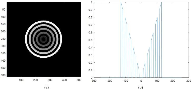
The aperture composed of ten cascaded black and linearly distributed function described in the 1st model is drawn as in the figure (1-a), where equal strips are assumed. The image has dimensions of 512×512 pixels while the aperture radius =
128 pixels. Five zones have linear distribution cascaded with another five dark zones starting from the center as dark. The Line plot of the described CBLD aperture is shown as in the figure (1-b), where ten zones are shown five of them has linear distribution cascaded with another black five zones.
Figure 1. (a): Design of the Cascaded Black-Linear Distribution (CBLD) in a circular aperture. The image has dimensions of 512× 512 pixels while the
In the 2nd model, Figure (2-a): Design of the Cascaded Black-Linear Distribution (CBLD) in a circular aperture. The image has dimensions of 512× 512 pixels while the aperture radius = 128 pixels. The aperture has twenty zones, where ten
zones have linear distribution cascaded with another ten dark zones starting from the center as dark. In addition, the line plot is shown as in the figure (2-b).
Figure 2. (a): Design of the Cascaded Black-Linear Distribution (CBLD) in a circular aperture. The image has dimensions of 512× 512 pixels while the
aperture radius = 128 pixels. Ten zones have linear distribution cascaded with another ten dark zones starting from the center as dark. (b): Line plot of the described CBLD aperture, shown in the figure (4-a), where twenty zones are shown ten of them has linear distribution cascaded with another black ten zones.
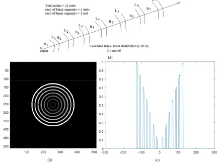
Figure 3. (a): The schematic representation of CBLD concentric annuli having a ratio 2:1 from the center. (b): Design of another Cascaded Black-Linear
Figure (3-a): The schematic representation of CBLD concentric annuli having a ratio 2:1 from the center. Design of the Cascaded Black-Linear Distribution (CBLD) in a circular aperture represented by the 3rd model is shown as in the figure (3-b). The image has dimensions of 512× 512 pixels while the aperture radius = 128 pixels. Seven zones have linear distribution cascaded with another seven dark zones starting with dark zone from the center. The ratio
between B and L zones is 2:1. The total number of zones N = 21. The Line plot of the CBLD of a ratio (where the center is assumed black) is plotted as in the figure (3-c).
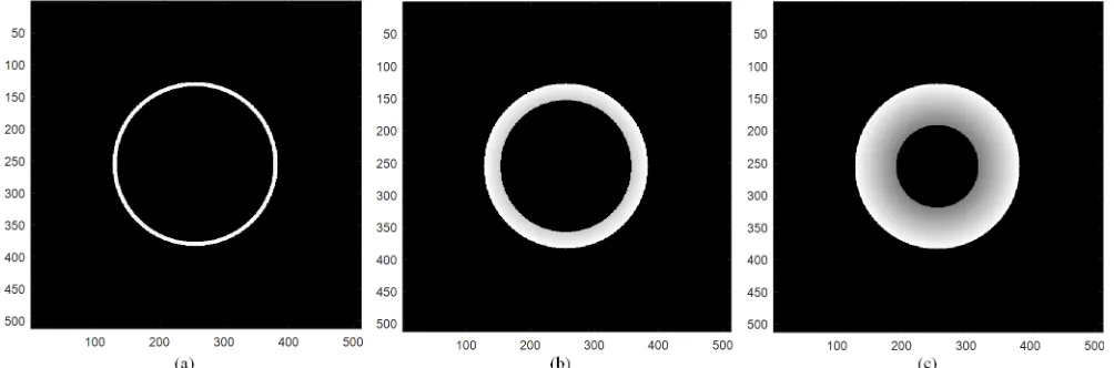
In the 4th model, annular aperture of linear distribution for different widths is shown in the figure (4 a-c). The annular width δρ = 0.05 as in the figure (4-a), δρ = 0.2 as in the figure (4-b), while two-layer thick annulus of aperture ratio 1:1 is shown as in the figure (4-c).
Figure 4. (a): A linearly distributed annular aperture of width = 0.05. (b): A linear annulus of moderate width = 0.2. (c): Two-layer thick annulus of aperture
ratio 1:1.
The PSF for the different models of CBLD apertures at different radii shown in the figures (5-8) are given in the Table 2, where the cut-off spatial frequency computed from the reduced coordinate is extracted from the different curves and the maximum amplitude at R = 16 pixels is shown.
Table 2. The PSF at radius=16 pixels corresponding to the different models and the deduced cut- off spatial frequencies and maximum amplitudes are given.
PSF at radius R = 16 pixels Number of zones (N) Cut-off spatial frequency (NA/lambda) r Maximum amplitude in pixels
Model 1 (CBLD) ratio 1:1 10 0.8111 291
Model 2 (CBLD) ratio 1:1 20 0.8111 303
Model 3 (CBLD) ratio 2:1 2×7+1×7= 21 0.8111 208
Model 4 linear annulus (width = 0.05) 2 0.6636 70
B/W transparent annuli (CBWD) 10 0.9586 431
It is shown, from the plots in the figures (5-8) and the table (2), that the cut-off spatial frequency for the linear annulus has the best resolution compared with the B/W transparent
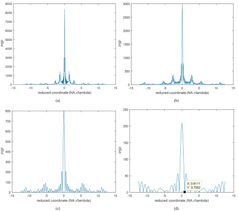
Figure 5. (a): Normalized PSF for the CBLD aperture shown in the figure 1, where the maximum radius = 128 pixels and the total number of zones N= 10. (b): Normalized PSF where the radius = 64 pixels. (c): Normalized PSF where the radius = 32 pixels. The cut-off spatial frequency is shown as: (NA. rc /lambda) = 0.4178. (d): The PSF where the radius = 16 pixels. PSF max. = 291 while the cut-off spatial frequency is shown as: (NA. rc /lambda) = 0.8111. The
legs of the diffraction pattern are strength like the ordinary B/W aperture while the resolution is better by an amount of 15.4%.
Figure 6. (a): The PSF for the CBLD aperture where radius = 128 pixels. where the total number of zones N = 20, as shown in the figure 2. (b): The PSF versus the reduced
Figure 7. (a): The PSF versus the reduced coordinate (NA/lambda) r corresponding to the model shown in the figure 3, where the ratio 2:1 is assumed for the CBLD. The radius = 128 pixels. (b): The PSF versus the reduced coordinate (NA/lambda) r. The radius = 64 pixels. (c): The PSF versus the reduced coordinate (NA/lambda) r. The radius = 32 pixels. (d): The PSF versus the reduced coordinate (NA/lambda) r. The radius = 16 pixels and N = 20. It is shown that PSF max.= 208 pixels while the cut-off spatial frequency is found to be: (NA. rc /lambda) = 0.8111.
(c)
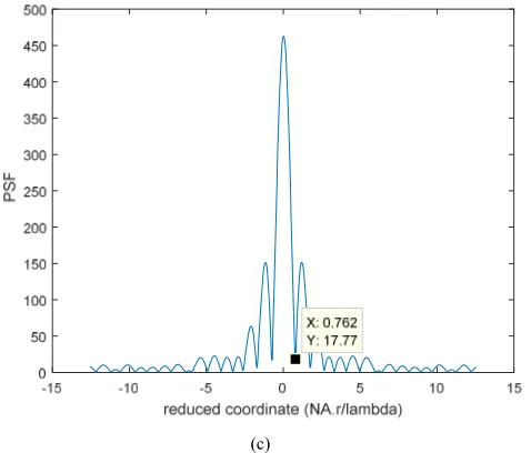
Figure 8. (a): PSF versus reduced coordinate. Width of the linear annulus =
0.05, external radius = 16 pixels as shown in the figure 4. (b): PSF versus reduced coordinate. Width of the linear annulus = 0.2, external radius = 16 pixels. (c): PSF versus reduced coordinate. Width of the linear annulus = 0.5, external radius = 16 pixels.
(a)
(b)
(c)
Figure 9. (a): The PSF for B/W transparent aperture where the radius = 16
pixels. PSF max. = 431 pixels while the cut-off spatial frequency is given as: (NA. rc /lambda) = 0.9586. The legs of the diffraction pattern are strength which is considered useful for imaging extended objects. (b): Normalized PSF for circular uniform aperture where the radius = 16 pixels. The cut-off spatial frequency is given as: (NA. rc /lambda) = 0.9586. (c): Normalized PSF for annular aperture of width = 5% from the total radius = 16 pixels. The cut-off spatial frequency is found to be: (NA. rc /lambda) = 0.6636. The intensity of the
diffracting spot is much decreased compared with the proposed model.
(a)
(c)
Figure 10. (a): PSF versus reduced coordinate. Width of the transparent
annulus = 0.05, external radius = 16 pixels. (b): PSF versus reduced coordinate. Width of the transparent annulus = 0.2, external radius = 16 pixels. (c): PSF versus reduced coordinate. Width of the transparent annulus = 0.5, external radius = 16 pixels.
(a)
(b)
(c)
(d)
(e)
P
S
(f)
(g)
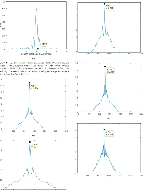
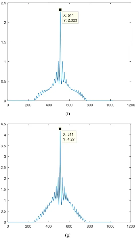
Figure 11. (a): CTF corresponding to CBLD aperture of equal zones (model
1). Total number of zones N = 10, CTF max = 3.704. CTF width = 2 aperture diameter = 512 pixels. (b): CTF using the FFT techniques. N = 10, CTF max = 2.419. (c): CTF corresponding to B/W concentric annuli of equal zones. Total number of zones N = 10. CTF max = 6.812. (d): CTF corresponding to CBLD aperture of equal zones (model 2). Total number of zones N = 20, CTF max = 3.228. CTF width = 2 aperture diameter = 512 pixels. (e): CTF corresponding to B/W concentric annuli of equal zones. Total number of zones N = 20. CTF max = 6.171. (f): CTF corresponding to CBLD aperture of ratio 2:1 (model 3). Total number of zones N = 21. CTF max = 2.323. (g): CTF corresponding to B/W concentric annuli of ratio 2:1. Total number of zones N = 21. CTF max = 4.27.
It is shown that the legs of the diffraction pattern in the PSF for the suggested models are stringent than the legs appeared for the uniform circular aperture which is useful for imaging extended objects.
In case of the CBLD models, the resolution is better by an amount of 15.4% as compared with the corresponding resolution in case of B/W transparent annuli. In addition, the maximum amplitude is increased while the total number N is increased. A value of 291 pixels is shown for N = 10 while a
value of 303 pixels is computed for N = 20. Equal ratio is assumed for the 1st two models while further increase of maximum amplitude to 354 pixels is attained for a ratio 1:2. In the 3rd model, contrast is further improved than the corresponding contrast in models 1, 2 for ratio 1:2 while it is decreased for ratio 2:1.
In the figure (10 a-c), the PSF plots is given for three different annuli where the legs of the diffraction pattern are appeared for smaller width.
The CTF computed for the three models of CBLD and compared with the CTF for B/W concentric annuli using equations (9) and (10). The CTF corresponding to all apertures are plotted as in the figure (11 a-f), and the peaks are computed and given in the table 3. The CTF is computed from the direct convolution product or the F. T techniques giving the same results.
The reconstructed images obtained corresponding to the CBLD aperture (model 1) are shown in the figure (12-a), compared with that obtained using B/W concentric annuli figure (12-b). Nearly, no difference is appeared in the two reconstructed images. The difference is outlined only as in the RPSF corresponding to the CBLD and the B/W arrangements as shown in the figures (5-d) and figure (9-a). It is shown an improvement of resolution in case of CBLD compared with the case of B/W apertures since rc (CBLD)=
0.8111 < rc (B/W)= 0.9586. Hence, reconstructed images in
case of CBLD is better in resolution compared with B/W concentric annuli for the same maximum radius.
(a)
(b)
Figure 12. (a): Reconstructed image using the CLSM provided with CBLD
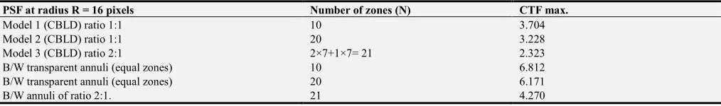
Table 3. CTF peaks corresponding to the three models of CBLD and B/W concentric annuli.
PSF at radius R = 16 pixels Number of zones (N) CTF max.
Model 1 (CBLD) ratio 1:1 10 3.704
Model 2 (CBLD) ratio 1:1 20 3.228
Model 3 (CBLD) ratio 2:1 2×7+1×7= 21 2.323
B/W transparent annuli (equal zones) 10 6.812
B/W transparent annuli (equal zones) 20 6.171
B/W annuli of ratio 2:1. 21 4.270
4. Conclusion
The suggested models of the CBLD apertures have compromised resolution and contrast compared with circular and annular transparent apertures. Contrast of the image will increase with the increase of the total number of concentric black and linear strips. CBLD has better resolution than the ordinary B/W transparent annuli and uniform circular apertures, hence the reconstructed images are better in resolution in case of CBLD. The suggested CBLD apertures have legs of reasonable amplitude which is useful in imaging extended objects as compared with the circular uniform aperture.
References
[1] M. Minsky, Microscopy Apparatus, United States Patent Office. Filed Nov. 7, 1957, granted Dec. 19, 1961. Patent No. 3, 013, 467 (1961).
[2] https://bitesizebio.com/19958/what-is-confocal-laser-scanning-microscopy/
[3] Sheppard, C. J. R., and Choudhury, A., 1977, Optica Acta, 24, 1051, Image Formation in the Scanning Microscope.
[4] Sheppard, C. J. R., 1986, J. Phys. D, 19, 2077, Scanned Imagery.
[5] Sheppard, C. J. R., and WILSON, T., 1978, Optica Acta, 25, 315 -325, Image Formation in Scanning Microscopes with Partially Coherent Source and Detector.
[6] Sheppard, C. J. R., Hamilton, D. K., and Cox, I. J., 1983, Proc. R. Soc., Lond. A, 387, 171.
[7] Sheppard, C. J. R., and Matthews, H. J., 1987, J. opt. Soc. Am., 4, 1354, Imaging in high-aperture optical systems. [8] Hopkins, H. H., 1955, Proc. R. Soc., Lond. A, 231, 91. [9] Levi, L., and Austing, R. H., 1968, Appl. Optics, 7, 967,
Determination of Equivalent Pass band of an aberration free lens using numerical methods.
[10] Cox, I. J., and Sheppard, C. J. R., 1986, J. opt. Soc. Am., 3, 1152-1158, Information capacity and resolution in an optical system.
[11] Egger, M. D., and Petran, M., 1967, Science, N. Y., 157, 305-307, New reflected-light microscope for viewing unstained brain and ganglion cells.
[12] Sheppard, C. J. R., and Wilson, T., 1981, J. Microsc., 124, 107, The theory of the direct‐view confocal microscope. [13] Sheppard, C. J. R., and Hamilton, D. K., 1984, Optica Acta,
31, 723.-727, Edge Enhancement by Defocusing of Confocal Images.
[14] Wilson, T.; Carlini, A. R. J. Microscopy 1988, 149, 51 –66, The effect of aberrations on the axial response of confocal imaging systems.
[15] Springer, K. R.; Fellers, T. J.; Davidson, M. W. Olympus Corporation; Florida State University: Tallahassee, FL, 2004. [16] Cox, G.; Sheppard, C. R. J. Microsc. Res. Tech. 2004, 63, 18–
22, Practical limits of resolution in confocal and non‐linear microscopy.
[17] Sheppard, C. J. R.; Shotton, D. M. Image Formation in the Confocal Laser Scanning Microscope; Springer-Verlag, New York Inc.: New York, 1997, pp. 15–31.
[18] Clair, J. J. & Hamed, A. M. (1983) 133-141, Theoretical studies on optical coherent microscopes. Optik 64 (2) 133-141.
[19] Hamed, A. M. and Clair, J. J. Optik 64 (1983) 277-284, Image and super-resolution in optical coherent microscopes.
[20] Hamed, A. M. and Clair, J. J. Optik 65 (1983) 209-218, Studies on optical properties of confocal scanning optical microscope using pupils with radially transmission distribution.
[21] Hamed, Opt. and laser technology 16 (1984) 93-96, Resolution and contrast in confocal optical scanning microscope.
[22] Sheppard, C. J. R., 1988, J. mod. Optics, 35, 145.
[23] Hamed, A. M. Precision Instrument and Mech. PIM 3 (2014) 144-152, Study of graded index and truncated apertures using speckle images.
[24] Hamed, A. M. and Al-Saeed, T. A. J. Modern Opt. 62 (2015) 801-810, Image analysis of modified Hamming aperture: application on confocal microscopy and holography.
[25] Hamed, A. M. Optik, 131 (2017) 838-849, Improvement of point spread function (PSF) using linear-quadratic aperture. [26] Sheppard, C. J. R. and Ma, X. Q., J. Modern Optics 35 (1988)
1169-1185, Confocal microscopes with slit apertures.