Probabilistic Couplings For Probabilistic Reasoning

University of Pennsylvania

ScholarlyCommons

Publicly Accessible Penn Dissertations

2017

Probabilistic Couplings For Probabilistic Reasoning

Justin Hsu

University of Pennsylvania, [email protected]

Follow this and additional works at:

https://repository.upenn.edu/edissertations

Part of the

Computer Sciences Commons

This paper is posted at ScholarlyCommons.https://repository.upenn.edu/edissertations/3017 For more information, please [email protected].

Recommended Citation

Hsu, Justin, "Probabilistic Couplings For Probabilistic Reasoning" (2017).Publicly Accessible Penn Dissertations. 3017.

Probabilistic Couplings For Probabilistic Reasoning

Abstract

This thesis explores proofs by coupling from the perspective of formal verification. Long employed in

probability theory and theoretical computer science, these proofs construct couplings between the output

distributions of two probabilistic processes. Couplings can imply various probabilistic relational properties,

guarantees that compare two runs of a probabilistic computation.

To give a formal account of this clean proof technique, we first show that proofs in the program logic pRHL

(probabilistic Relational Hoare Logic) describe couplings. We formalize couplings that establish various

probabilistic properties, including distribution equivalence, convergence, and stochastic domination. Then we

deepen the connection between couplings and pRHL by giving a proofs-as-programs interpretation: a

coupling proof encodes a probabilistic product program, whose properties imply relational properties of the

original two programs. We design the logic xpRHL (product pRHL) to build the product program, with

extensions to model more advanced constructions including shift coupling and path coupling.

We then develop an approximate version of probabilistic coupling, based on approximate liftings. It is known

that the existence of an approximate lifting implies differential privacy, a relational notion of statistical privacy.

We propose a corresponding proof technique---proof by approximate coupling---inspired by the logic apRHL,

a version of pRHL for building approximate liftings. Drawing on ideas from existing privacy proofs, we extend

apRHL with novel proof rules for constructing new approximate couplings. We give approximate coupling

proofs of privacy for the Report-noisy-max and Sparse Vector mechanisms, well-known algorithms from the

privacy literature with notoriously subtle privacy proofs, and produce the first formalized proof of privacy for

these algorithms in apRHL.

Finally, we enrich the theory of approximate couplings with several more sophisticated constructions: a

principle for showing accuracy-dependent privacy, a generalization of the advanced composition theorem

from differential privacy, and an optimal approximate coupling relating two subsets of samples. We also show

equivalences between approximate couplings and other existing definitions. These ingredients support the

first formalized proof of privacy for the Between Thresholds mechanism, an extension of the Sparse Vector

mechanism.

Degree Type

Dissertation

Degree Name

Doctor of Philosophy (PhD)

Graduate Group

Computer and Information Science

First Advisor

Second Advisor

Aaron Roth

Subject Categories

PROBABILISTIC COUPLINGS

FOR PROBABILISTIC REASONING

Justin Hsu

A DISSERTATION

in

Computer and Information Science

Presented to the Faculties of the University of Pennsylvania in Partial

Fulfillment of the Requirements for the Degree of Doctor of Philosophy

2017

Benjamin C. Pierce, Professor of Computer and Information Science Co-supervisor of Dissertation

Aaron Roth, Associate Professor of Computer and Information Science Co-supervisor of Dissertation

Lyle Ungar, Professor of Computer and Information Science Graduate Group Chairperson

Dissertation Committee

Gilles Barthe, Research Professor, IMDEA Software Institute

Sampath Kannan, Professor of Computer and Information Science

Val Tannen, Professor of Computer and Information Science

PROBABILISTIC COUPLINGS FOR PROBABILISTIC REASONING COPYRIGHT © 2017 Justin Hsu

Typeset in Charter and Math Design with LA_TEX.

Acknowledgments

It takes a village, as they say. I am extremely fortunate to have two amazing advisers: Benjamin Pierce, who taught me to ponder slowly, and Aaron Roth, who taught me to think rapidly. This thesis would not have existed without Gilles Barthe, serving as a third, unofficial adviser. Gilles hosted me during two highly productive summers at the IMDEA Software Institute in Madrid and remains an inspiring (and boundless) source of energy and enthusiasm. He and his longtime collaborators, Pierre-Yves Strub and Benjamin Grégoire, provided a wealth of technical expertise and a theoretical setting that turned out to be far richer than anyone had thought.

The strong theory and formal methods faculty at Penn, including Sanjeev Khanna, Stephanie Weirich, Michael Kearns, Steve Zdancewic, Sampath Kannan, Val Tannen, Sudipto Guha, and Rajeev Alur, have taught me more than I can hope to remember. I am also indebted to Marco Gaboardi and Emilio Jesús Gallego Arias for launching me to the research frontiers. Other fellow students and postdocs, including Arthur Azevedo de Amorim, Rachel Cummings, Michael Greenberg, Radoslav Ivanov, Shahin Jabbari, Matthew Joseph, Jamie Morgenstern, Christine Rizkallah, Ryan Rogers, Nikos Vasilakis, and Steven Wu, kept morale at a good level, to say the least.

At Stanford, Greg Lavender’s one-off course on Haskell gave me my first glimpse of programming languages as an intellectual field. Without that formative experience, I never would have gone on to graduate school in computer science. Finally, I am deeply grateful for the constant support and encouragement from my parents Joyce and David, my sister Tammy, and the rest of my family.

ABSTRACT

PROBABILISTIC COUPLINGS FOR PROBABILISTIC REASONING

Justin Hsu

Benjamin C. Pierce and Aaron Roth

This thesis exploresproofs by couplingfrom the perspective of formal verification. Long employed in

probability theory and theoretical computer science, these proofs constructcouplingsbetween the output

distributions of two probabilistic processes. Couplings can imply variousprobabilistic relational properties,

guarantees that compare two runs of a probabilistic computation.

To give a formal account of this clean proof technique, we first show that proofs in the program

logic PRHL (probabilistic Relational Hoare Logic) describe couplings. We formalize couplings that

establish various probabilistic properties, including distribution equivalence, convergence, and stochastic

domination. Then we deepen the connection between couplings andPRHL by giving a proofs-as-programs

interpretation: a coupling proof encodes a probabilisticproduct program, whose properties imply relational

properties of the original two programs. We design the logic×PRHL (productPRHL) to build the product

program, with extensions to model more advanced constructions includingshift couplingandpath coupling.

We then develop an approximate version of probabilistic coupling, based onapproximate liftings. It

is known that the existence of an approximate lifting impliesdifferential privacy, a relational notion of

statistical privacy. We propose a corresponding proof technique—proof by approximate coupling—inspired

by the logicAPRHL, a version ofPRHL for building approximate liftings. Drawing on ideas from existing

privacy proofs, we extendAPRHL with novel proof rules for constructing new approximate couplings.

We give approximate coupling proofs of privacy for theReport-noisy-maxandSparse Vectormechanisms,

well-known algorithms from the privacy literature with notoriously subtle privacy proofs, and produce

the first formalized proof of privacy for these algorithms inAPRHL.

Finally, we enrich the theory of approximate couplings with several more sophisticated constructions: a

principle for showing accuracy-dependent privacy, a generalization of the advanced composition theorem

from differential privacy, and an optimal approximate coupling relating two subsets of samples. We also

show equivalences between approximate couplings and other existing definitions. These ingredients

support the first formalized proof of privacy for theBetween Thresholdsmechanism, an extension of the

Contents

1 Introduction 1

1.1 Challenges in probabilistic reasoning . . . 1

1.2 Couplings and relational properties. . . 2

1.3 A formal study of proofs by coupling . . . 3

2 Couplings à la formal verification 5 2.1 Mathematical preliminaries. . . 5

2.2 A formal logic for coupling proofs. . . 11

2.3 Constructing couplings, formally . . . 19

2.4 Related work. . . 23

3 From coupling proofs to product programs 25 3.1 The core logic×PRHL . . . 25

3.2 An asynchronous loop rule . . . 29

3.3 Soundness of the logic. . . 31

3.4 Proving probabilistic convergence. . . 31

3.5 Shift couplings . . . 33

3.6 Path couplings. . . 37

3.7 Comparison with existing product programs . . . 42

4 Approximate couplings for privacy 44 4.1 Differential privacy preliminaries . . . 44

4.2 Approximate liftings . . . 46

4.3 The program logicAPRHL. . . 52

4.4 Proof by approximate coupling . . . 55

4.5 New couplings for the Laplace distribution . . . 56

4.6 Pointwise privacy . . . 59

4.7 Coupling proofs of privacy . . . 61

4.8 Discussion . . . 69

5 Advanced approximate couplings 73 5.1 Equivalence with Sato’s approximate lifting. . . 73

5.2 Accuracy-dependent approximate couplings . . . 81

5.3 Optimal subset coupling. . . 85

5.4 Advanced coupling composition . . . 89

5.5 Proving privacy for Between Thresholds . . . 96

5.6 Comparison to other approximate liftings . . . 101

6 Emerging directions 107 6.1 Concurrent developments. . . 107

6.3 Bridging two theories . . . 112

A Soundness of×PRHL 113

B Soundness ofAPRHL 124

List of Figures

2.1 Semantics of programs . . . 13

2.2 Two-sidedPRHL rules . . . 15

2.3 One-sidedPRHL rules . . . 17

2.4 StructuralPRHL rules . . . 18

3.1 Two-sided×PRHL rules . . . 27

3.2 One-sided×PRHL rules . . . 28

3.3 Structural×PRHL rules . . . 29

3.4 Asynchronous loop rule_[WHILE-GEN]for×PRHL . . . 29

4.1 Two-sidedAPRHL rules . . . 53

4.2 One-sidedAPRHL rules . . . 54

4.3 StructuralAPRHL rules . . . 55

4.4 New Laplace rules forAPRHL . . . 56

4.5 Pointwise equality rule[PW-EQ]forAPRHL . . . 60

4.6 Sparse Vector. . . 65

5.1 Up-to-bad rules forAPRHL. . . 84

5.2 One-sided conjunction rules forAPRHL . . . 84

5.3 Laplace accuracy bounds inAPRHL . . . 85

5.4 Interval coupling rule[LAPINT]forAPRHL . . . 87

5.5 Conversion rules between symmetric and standard judgments forAPRHL. . . 94

5.6 Advanced composition rule[WHILE-AC]forAPRHL . . . 94

Chapter 1

Introduction

Randomized algorithms have long stimulated the imagination of computer scientists. Endowed with the power to draw random samples, these algorithms provide sophisticated guarantees far beyond the reach of deterministic computations. However, their proofs of correctness are often highly intricate, employing specialized techniques to reason about randomness.

This thesis investigates one such tool—probabilistic coupling—for provingprobabilistic relational properties, which compare executions of two randomized algorithms. Couplings are a familiar concept in probability theory and theoretical computer science, where they support a proof technique called

proof by coupling. We explore the reasoning principle behind these proofs, identifying their theoretical underpinnings, clarifying their structure, and enabling formal verification.

1.1

Challenges in probabilistic reasoning

While probabilistic programs aren’t much harder to express than their deterministic counterparts, they are significantly more challenging to reason about. To see why, suppose we want to prove a property about the output of an algorithm for all inputs. In a deterministic algorithm, each concrete input produces a single trace through the program. Since different paths correspond to distinct inputs, we can freely group similar traces together and reason about each group on its own. The code of the algorithm naturally guides the proof: at a branching instruction, for instance, we may classify the executions according to the path they take and then consider each behavior separately. In this way, we can reason about a complex program by focusing on simpler cases.

For randomized algorithms, this neat picture is considerably more complicated. A single execution now comprises multiple traces, each with its own probability. Relations between trace probabilities make it difficult to reason about paths separately. At a conditional statement, for instance, the execution has some probability of taking the first branch and some probability of taking the second branch; in a sense, the computation takesbothbranches. If we reason about these two cases in isolation, we must track the probabilities of each branch in order to join the cases when the paths later merge. This is challenging even for small programs, as a path’s probability can have complex dependencies on the input and on the probabilities of other possible traces. If we instead reason about both behaviors together, we must provide a single analysis for executions that behave quite differently.

support proofs for a broad class of properties. A proof technique is a reusable component for analyzing algorithms, and is as much of an intellectual contribution as any new proof or algorithm.

1.2

Couplings and relational properties

In this thesis we explore a proof technique forprobabilistic relational properties, guarantees comparing the runs of two randomized algorithms. Such properties are commonplace in computer science and probability theory. Examples include:

• Probabilistic equivalence: two probabilistic programs produce equal distributions.

• Stochastic domination: one probabilistic program is more likely than another to produce large outputs.

• Convergence (alsomixing): the output distributions of two probabilistic loops approach each other as the loops execute more iterations.

• Indistinguishability(alsodifferential privacy): the output distributions of two probabilistic pro-grams are close together. For instance,differential privacyrequires that two similar inputs—say, the real private database and a hypothetical version with one individual’s data omitted—yield similar output distributions.

• Truthfulness(alsoNash equilibrium): an agent’s average utility is larger when reporting an honest value instead of deviating to a misleading value.

At first glance, relational properties appear to be even harder to establish than standard, non-relational properties—instead of analyzing a single probabilistic computation, we now need to deal with two. (Indeed, any property of a single program can be viewed as a relational property between the target program and the trivial, do-nothing program.) However, relational properties often relate two highly similar programs, even comparing the same program on two possible inputs. In these cases, we can leverage a powerful abstraction and an associated proof technique from probability theory—probabilistic couplingandproof by coupling.

The fundamental observation is that probabilistic relational properties compare computations in two different worlds, assuming no particular correlation between random samples. Accordingly, we may freely assume any correlation we like for the purposes of the proof—a relational property holds (or doesn’t hold) regardless of which one we pick. For instance, if two programs generate identical output distributions, this holds whether they share coin flips or take independent samples; relational properties don’t require that the two programs use separate randomness. By carefully arranging the correlation, we can reason about two executions as if they were linked in some convenient way.

To take advantage of this freedom, we need some way to design specific correlations between program executions. In principle, this can be a highly challenging task. The two runs may take samples from different distributions, and it is unclear exactly how they can or should share randomness. When the two programs have similar shapes, however, we can link two computations in a step-by-step fashion. First, correlations between intermediate samples can be described byprobabilistic couplings, joint distributions over pairs. For example, a valid coupling of two fair coin flips could specify that the draws take opposite values; the correlated distribution would produce “(heads, tails)” and “(tails, heads)” with equal probability. A coupling formalizes what it means to share randomness: a single source of randomness simulates draws from two distributions. Since randomness can be shared in different ways, two distributions typically support a variety of distinct couplings.

remain opposite when analyzing the rest of the programs. By flowing these relations forward from two initial inputs, a proof by coupling can focus on just pairs of similar executions as it builds up to a coupling between two output distributions. This is the main product of the proof: features of the final coupling imply properties about the output distributions, and hence relational properties about the original programs.

Working in tandem, couplings and proofs by couplings can simplify probabilistic reasoning in several ways.

• Reduce to one source of randomness. By analyzing two runs as if they shared a single source of randomness, we can reason about two programs as if they were one.

• Abstract away probabilities. Proofs by coupling isolate probabilistic reasoning from the non-probabilistic parts of the proof, which are more straightforward. We only need to think about probabilistic aspects when we select couplings at the sampling instructions; throughout the rest of the programs, we can reason purely in terms of deterministic relations between the two runs.

• Enable compositional, structured reasoning.By focusing on each step of an algorithm individ-ually and then smoothly combining the results, the coupling proof technique enables a highly modular style of reasoning guided by the code of the program.

Proofs by coupling are also surprisingly flexible; many probabilistic relational properties, including the examples listed above, can be proved in this way. Individual couplings can also be combined in various subtle ways, giving rise to a rich diversity of coupling proofs.

1.3

A formal study of proofs by coupling

While couplings proofs originate from probability theory as a tool for human reasoning,formal verification

will be the setting for our investigation. Our perspective affords two distinct advantages.

• The theory of formal verification provides a wealth of concepts to precisely describe and analyze proof systems. By studying coupling proofs in these terms, we can give a fresh understanding of this classical proof technique. As a consequence, we can extend proofs by coupling to target new guarantees, unifying seemingly unrelated properties and simplifying their proofs.

• Formal verification systems provide a natural domain to apply our insights. First, couplings enable clean proofs for properties that are traditionally challenging for computers to verify. Existing techniques can also be considered in a new light, clarifying why certain features are useful and revealing possible enhancements.

The technical chapters of this thesis fall into two parts. Chapters 2 and3 concern probabilistic couplings, while Chapters4and5investigate approximate couplings. General themes and intuitions developed in the first half influence the second half, but the two parts are largely self-contained and can be read independently.

Chapter2begins our study of probabilistic couplings in formal verification. We observe that the program logicPRHL (probabilistic Relational Hoare Logic), originally proposed byBarthe, Grégoire, and Zanella-Béguelin(2009) for verifying proofs of cryptographic security, is in fact a logic for formally con-structing probabilistic couplings. Using this connection, we formalize classical coupling proofs establishing equivalence, convergence, and stochastic domination of probabilistic processes.

Chapter3deepens our correspondence between couplings andPRHL. First, coupling proofs describe how to meld two probabilistic programs into a single program; in formal verification, such a construction is known as aproduct program. Accordingly, we show thatPRHL proofs encode a novel kind of product program called thecoupled product, reflecting the structure of a coupling proof. This idea recalls a central theme in logic and computer science: formal proofs can be interpreted as computations, a so-called

(productPRHL) that constructs the product program alongside the coupling proof. Then, we design a new loop rule inspired byshift coupling, a way to build couplings asynchronously. As applications, we formalize rapid mixing for several Markov chains. Our approach can also capture a simplified version of thepath couplingtechnique introduced byBubley and Dyer(1997).

Chapter4turns our focus to a generalization of couplings:approximate couplings. These couplings are closely related todifferential privacy, a quantitative, relational property modeling statistical privacy. We begin with a candidate definition of approximate coupling, refining several existing notions. We then reverse-engineer a corresponding proof technique calledproof by approximate couplingfrom the program logicAPRHL, an approximate version ofPRHL proposed byBarthe, Köpf, Olmedo, and Zanella-Béguelin

(2013c). Taking inspiration from this proof technique, we show how two new approximate couplings of the Laplace distribution and a construction calledpointwise equalityenable an approximate coupling proof of privacy for theReport-noisy-maxandSparse Vectormechanisms. Our proofs are simpler than existing proofs—which were notoriously difficult to get right (Lyu, Su, and Li,2017)—and extend to natural variants of the algorithms. We realize our proof in an extension ofAPRHL, arriving at the first formalized privacy proofs for these mechanisms.

Chapter5presents a handful of advanced constructions for approximate couplings: (i) a principle for proving accuracy-dependent privacy; (ii) a construction for linking two subsets of samples; and (iii) a composition principle generalizing the advanced composition theorem from differential privacy. We also clarify the landscape of existing definitions by proving equivalences between approximate couplings and prior notions of approximate equivalence. Combining these ingredients, we give a proof by approximate coupling establishing differential privacy for theBetween Thresholdsmechanism byBun, Steinke, and Ullman(2017). After extendingAPRHL with several rules corresponding to our constructions, we achieve the first formalized privacy proof for this algorithm.

Chapter6surveys concurrent work on couplings and formal verification, outlining promising directions for further developing the theory and application of proofs by coupling.

A note about mechanical verification. The gold standard in formal verification ismechanized proof, where every step has been fully computer-checked. The logics we will develop are highly suitable for computer verification, due to their highly structured proofs, but we do not mechanically verify coupling proofs as part of this thesis. Instead, we will describeformalized proofsin the logic on paper. Prototype implementations in the EASYCRYPTframework (Barthe, Dupressoir, Grégoire, Kunz, Schmidt, and Strub,

2013b) can machine-check versions of the coupling proofs we will see (see, e.g.,Barthe et al.(2013c) andBuch(2017)), but the current implementations are not precisely aligned with our logics.

Acknowledgments. The technical content of this thesis draws on a fruitful collaboration with Gilles Barthe, Thomas Espitau, Noémie Fong, Marco Gaboardi, Benjamin Grégoire, Tetsuya Sato, Léo Stefanesco and Pierre-Yves Strub. Chapter2is based onBarthe, Espitau, Grégoire, Hsu, Stefanesco, and Strub

Chapter 2

Couplings à la formal verification

To begin our formal investigation of coupling proofs, we first provide the necessary mathematical back-ground (Section2.1), and then draw a deep connection between coupling proofs and the program logic

PRHL (Section2.2); this observation is the principal conceptual contribution of this chapter and forms the foundation for the entire thesis. We show how to formalize several examples of couplings (Section2.3), and discuss related work on relational program logics and probabilistic liftings (Section2.4).

2.1

Mathematical preliminaries

A discrete probability distribution associates each element of a set with a number in[0, 1], representing itsprobability. In order to model programs that may not terminate, we work with a slightly more general notion called asub-distribution.

Definition 2.1.1. A (discrete)sub-distributionover a countable setAis a map_µ:A→[0, 1_]taking each element ofAto a numeric weight such that the weights sum to at most 1:

X

a∈A

µ(a)≤1.

We writeSDistr₍A)for the set of all sub-distributions overA. When the weights sum to 1, we call_µa

properdistribution; we writeDistr₍A)for the set of all proper distributions overA. Theemptyornull sub-distribution⊥assigns weight 0 to all elements.

We work with discrete sub-distributions throughout. While this is certainly a restriction—excluding, for instance, standard distributions over the real numbers—many interesting coupling proofs can already be expressed in our setting. Where necessary, we will use discrete versions of standard, continuous distributions. Our results should mostly carry over to the continuous setting, as couplings are frequently used on continuous distributions in probability theory, but the general case introduces measure-theoretic technicalities (e.g., working with integrals rather than sums, checking sets are measurable, etc.) that would distract from our primary focus. We discuss this issue further in Chapter6.

We need several concepts and notations related to discrete distributions. First, the probability of a set

S⊆A:

µ(S)¬

X

a∈S µ(a).

Thesupportof a sub-distribution is the set of elements with positive probability:

supp(µ)¬{a∈A|µ(a)>0}.

Theweightof a sub-distribution is the total probability of all elements:

|µ|¬

X

Sub-distributions can be ordered pointwise:µ₁≤µ2ifµ1(a)≤µ2(a)for every elementa∈A. Finally,

given a function f :A_→BwhereBis numeric (like the integers or the reals), itsexpected valueover a sub-distributionµis

E_µ[f]¬ E_a

∼µ[f(a)]¬

X

a∈A

f(a)·µ(a).

Under light assumptions, the expected value is guaranteed to exist (for instance, whenf is a bounded function).

To transform sub-distributions, we can lift a function f :A_→Bon sets to a map f]:SDistr(A)_→ SDistr(B)via f](µ)(b)¬µ(f−1(b)). For example, letp1:A1×A2→A1andp2:A1×A2→A2be the

first and second projections from a pair. The correspondingprobabilistic projectionsπ₁:SDistr(A_1×A2)_→ SDistr(A1)andπ₂:SDistr(A_1×A2)_→SDistr(A2)are defined by

π1(µ)(a1)_¬p]₁(µ)(a1) = X a2∈A2

µ(a₁,a2)

π2(µ)(a2)¬p]₂(µ)(a2) =

X

a1∈A1

µ(a₁,a2).

We call a sub-distribution_µover pairs ajoint sub-distribution, and the projected sub-distributions_π1(µ) and_π2(µ)thefirstandsecond marginals, respectively.

Probabilistic couplings and liftings

A probabilistic coupling models two distributions with a single joint distribution.

Definition 2.1.2. Givenµ₁,µ₂sub-distributions overA₁andA₂, a sub-distributionµover pairsA_1×A₂

is acouplingfor(µ1,µ2)ifπ1(µ) =µ1andπ2(µ) =µ2.

Generally, couplings are not unique—different witnesses represent different ways to share randomness between two distributions. To give a few examples, we first introduce some standard distributions.

Definition 2.1.3. LetAbe a finite, non-empty set. Theuniform distributionoverA, writtenUnif(A), assigns probability 1/|A_|to each element. We writeFlipfor the uniform distribution over booleans, the distribution of a fair coin flip.

Example 2.1.4(Couplings from bijections). We can give two distinct couplings of(Flip,Flip):

Identity coupling:

µid(a₁,a2)¬

¨

1/2 :a₁=a₂

0 : otherwise.

Negation coupling:

µ¬(a1,a2)¬

¨

1/2 :¬a₁=a₂

0 : otherwise.

More generally, any bijectionf :A→Ayields a coupling of(Unif(A),Unif(A)):

µf(a1,a2)¬

¨

1_/|A| :f(a1) =a₂

0 : otherwise.

For more general distributions, ifa₁anda₂have different probabilities underµ₁andµ₂then the correlated distribution cannot return(a₁,−)and(−,a2)with equal probabilities; for instance, a bijection with f(a1) =a₂would not give a valid coupling. However, general distributions can be coupled in other ways.

Example 2.1.5. Letµbe a sub-distribution overA. Theidentity couplingof(µ,µ)is

µid(a1,a2)¬

¨

µ(a) :a₁=a₂=a

0 : otherwise.

Sampling from this coupling yields a pair of equal values.

Example 2.1.6. Letµ₁,µ₂be sub-distributions overA₁andA₂. Theindependentortrivialcoupling is

µ×(a1,a2)¬µ1(a1)·µ2(a2).

This coupling modelsµ1andµ2as independent distributions: sampling from this coupling is equivalent

to first sampling fromµ1and then pairing with a fresh draw fromµ2. The coupled distributions must be

proper in order to ensure the marginal conditions.

Since any two proper distributions can be coupled by the trivial coupling, the mere existence of a coupling yields little information. Couplings are more useful when the joint distribution satisfies additional conditions, for instance when all elements in the support satisfy some property.

Definition 2.1.7(Lifting). Letµ1,µ2be sub-distributions overA1andA2, and letR⊆A1×A2be a

relation. A sub-distributionµover pairsA₁×A₂is awitnessfor theR-liftingof(µ1,µ2)if:

1. µis a coupling for(µ1,µ2), and

2. supp(µ)⊆R.

If there existsµsatisfying these two conditions, we sayµ₁andµ₂are related by thelifting ofRand write

µ1R]µ2.

We typically expressRusing set notation, i.e.,

R=_{(a₁,a2)_∈A_1×A_2|Φ(a₁,a2)_}

whereΦis a logical formula. WhenΦis a standard mathematical relation (e.g., equality), we leaveA₁

andA₂implicit and just writeΦ, sometimes enclosed by parentheses(Φ)for clarity.

Example 2.1.8. Many of the couplings we saw before are more precisely described as liftings.

Bijection coupling. For a bijectionf :A_→A, the coupling in Example2.1.4witnesses the lifting

Unif(A)_{(a₁,a2)_|f(a1) =a_2}]Unif(A).

Identity coupling. The coupling in Example2.1.5witnesses the lifting

µ(=)]_µ.

Trivial coupling. The coupling in Example2.1.6witnesses the lifting

µ1>]µ2.

(>¬A1×A2is the trivial relation relating all pairs of elements.)

Useful consequences of couplings and liftings

If there exists a couplingµbetween(µ1,µ2)satisfying certain properties, we can deduce probabilistic

properties aboutµ1andµ2. First of all, two coupled distributions have equal weight.

Proposition 2.1.9(Equality of weight). Supposeµ₁andµ₂are sub-distributions overAsuch that there exists a couplingµofµ₁andµ₂. Then|µ1|=|µ2|.

This follows becauseµ1andµ2are both projections ofµ, and projections preserve weight. Couplings

can also show that two distributions are equal.

Proposition 2.1.10(Equality of distributions). Supposeµ₁andµ₂are sub-distributions overA. Then µ1=µ2if and only if there is a liftingµ1(=)]µ2.

Proof. For the forward direction, defineµ(a,a)¬µ1(a) =µ2(a)andµ(a1,a2)¬0 otherwise. Evidently, µhas support in the equality relation(=)and also has the desired marginals:π1(µ) =µ1andπ2(µ) =µ2.

Thusµis a witness to the desired lifting.

For the reverse direction, let the witness be_µ. By the support condition,_π1(µ)(a) =π2(µ)(a)for everya∈A. Since the left and right sides are equal to_µ1(a)and_µ2(a)respectively by the marginal conditions,µ1(a) =µ2(a)for everya. So,µ₁andµ₂are equal.

In some cases we can show results in the converse direction: if a property of two distributions holds, then there exists a particular lifting. To give some examples, we first introduce a powerful equivalence due toStrassen(1965).

Theorem 2.1.11. Letµ₁,µ₂be sub-distributions overA₁andA₂, and letRbe a binary relation overA₁ andA₂. Then the liftingµ₁R]µ₂impliesµ1(S1)_≤µ2(R(S1))for every subsetS_1⊆A₁, whereR(S1)_⊆A₂ is theimageofS₁underR:

R(S1)_¬{a₂∈A_{2| ∃}a₁∈A₁, (a₁,a2)∈R_}.

(For instance, ifA₁=A₂=NandRis the relation≤, thenR(S)is the set of all natural numbers larger

thanminS.) The converse holds ifµ₁andµ₂have equal weight.

Strassen proved Theorem2.1.11for continuous (proper) distributions using deep results from proba-bility theory. In our discrete setting, there is an elementary proof by the maximum flow-minimum cut theorem; the proof also establishes a mild generalization to sub-distributions. So as not to interrupt the flow here, we defer details of the proof to Chapter5. For now, we use this theorem to illustrate a few more useful consequences of liftings. For starters, couplings can bound the probability of an event in the first distribution by the probability of an event in the second distribution.

Proposition 2.1.12. Supposeµ₁,µ₂are sub-distributions overA₁andA₂respectively, and consider two subsetsS_1⊆A₁andS_2⊆A₂. The lifting

µ1{(a1,a2)|a1∈S1→a2∈S2}]µ2

impliesµ1(S1)_≤µ2(S2). The converse holds whenµ₁andµ₂have equal weight.

Proof. LetRbe the relation {(a₁,a2)|a₁ ∈S_{1 →}a₂∈S_2}. The forward direction is immediate by Theorem2.1.11, taking the subsetS₁. For the reverse direction, consider any non-empty subsetT_1⊆A₁. IfT₁is not contained inS₁, thenR(T1) =A₂andµ1(T1)_≤µ2(R(T1))sinceµ₁andµ₂have equal weight. OtherwiseR(T1) =S₂, so

µ1(T1)_≤µ1(S1)_≤µ2(S2) =µ2(R(T1)). Theorem2.1.11gives the desired lifting:

A slightly more subtle consequence isstochastic domination, an order on distributions over an ordered set.

Definition 2.1.13. Let(A,≤A)be an ordered set and supposeµ1,µ2are sub-distributions overA. We

sayµ2stochastically dominatesµ1, denotedµ1≤sdµ2, if

µ1({a_∈A_|k_≤Aa})≤µ2({a∈A|k≤Aa})

for everyk∈A.

This order is different from the pointwise order on sub-distributions since it uses the order on the underlying space. For instance, two proper distributions satisfyµ1≤µ2exactly whenµ1=µ2, but two

unequal distributions may satisfy_µ1≤sd µ2; e.g., if we take distributions over the natural numbersN

with the usual order and_µ1places weight 1 on 0 while_µ2places weight 1 on 1. Stochastic domination is precisely the probabilistic lifting of the order relation.

Proposition 2.1.14. Supposeµ₁,µ₂ are sub-distributions over a set A with a reflexive order ≤A (i.e.,

a≤Aa). Thenµ1(≤A)]µ2impliesµ1≤sdµ2. The converse also holds whenµ1andµ2have equal weight, as long as any upwards closed subset ofAeither contains a minimum element or is the whole setA(e.g., A=_Nor_Zwith the usual order).

Proof. LetR¬(≤A). For the forward direction, Theorem2.1.11gives

µ1({a∈A|k≤Aa})≤µ2(R({a∈A|k≤Aa})).

The subset on the right is precisely the set ofa0∈Asuch thata0≥Aafor somea≥Ak; by transitivity and reflexivity, we have

µ2(R(_{a_∈A_|k_≤Aa_})) =µ2(_{a_∈A_|k_≤Aa_}).

This holds for allk_∈A, establishingµ1≤sdµ2.

For the converse, supposeµ1≤sdµ2andµ1andµ2have equal weights, and letS⊆Abe any subset.

If the upwards closureR(S)is the whole setA, thenµ1(S)_≤µ2(R(S))sinceµ1 andµ2have equal

weights. Otherwise, there is a least elementkofR(S)by assumption, and we have

µ1(S)≤µ1(R(S)) =µ1({a∈A|k≤Aa})≤µ2({a∈A|k≤Aa}) =µ2(R(S)),

where the middle inequality is by stochastic domination. Theorem2.1.11implies_µ1(≤A)]µ2.

Finally, a typical application of coupling proofs is showing that two distributions are close together.

Definition 2.1.15. Letµ1,µ2be sub-distributions overA. Thetotal variation distance(also known as TV-distanceorstatistical distance) betweenµ1andµ2is defined as

d_tv(µ₁,_µ2)¬1

2

X

a∈A

|µ1(a)−µ2(a)|=max

S⊆A|µ1(S)−µ2(S)|.

In particular, the total variation distance bounds the difference in probabilities of any event.

Couplings are closely related to TV-distance.

Theorem 2.1.16(see, e.g.,Levin, Peres, and Wilmer(2009);Lindvall(2002)). Letµ₁andµ₂be sub-distributions overAand letµbe a coupling. Then

d_tv(µ₁,µ2)≤ Pr

(a1,a2)∼µ

In particular, ifµwitnesses the lifting

µ1{(a1,a2)∈A×A|(a1,a2)∈S→a1=a2}]µ2,

then the TV-distance is bounded by the probability

d_tv(µ₁,µ2)≤ Pr

(a₁,a₂)∼µ[(a1,a2)∈/S].

Theorem 2.1.16is the fundamental result behind the so-calledcoupling method (Aldous,1983), a technique to show two probabilistic processes converge by constructing a coupling that causes the processes to become equal with high probability.1 _{This theorem is usually stated for proper distributions} µ1andµ2; the result on sub-distributions follows as an easy consequence. (If there is a lifting thenµ1

andµ₂have equal weightswby Proposition2.1.9, and the inequalities in Theorem2.1.16are preserved whenµ₁andµ₂are scaled by the same constant. Whenw=0 the inequality is immediate; otherwise, by scaling up both distributions by 1/w, applying the standard theorem to obtain the total variation bound for proper distributions, then scaling back down byw, we recover the total variation bound for sub-distributions.) Unlike the previous facts, the target property aboutµ1andµ2does not directly follow

from the existence of a lifting—we need more detailed information about the couplingµ.

Proof by coupling

The previous results suggest an indirect approach to proving properties of two distributions: demonstrate there exists a coupling of a particular form. However, how are we supposed to find a witness distribution with the desired properties? The given distributions may be highly complex, possibly over infinite sets—it is not clear how to represent, much less construct, the desired coupling.

To address this challenge, probability theorists have developed a powerful proof technique calledproof by coupling. This technique assumes a bit more information about the distributions: we need concrete descriptions of two processesproducingthe distributions. Usually, these generating programs are readily available; indeed, they are often the most natural descriptions of complex distributions.

Given two programs, a proof by coupling builds a coupling for the output distributions by coupling intermediate samples. In a bit more detail, we imagine stepping through the programs in parallel, one instruction at a time, starting from two inputs. Whenever we reach two corresponding sampling instructions, we pick a valid coupling for the sampled distributions. The selected couplings induce a relation on samples, which we can assume when analyzing the rest of the programs. For instance, by selecting couplings for earlier samples carefully, we may be able to assume the coupled programs take the same path at a subsequent branching statement; in this way, coupling proofs can consider just pairs of well-behaved executions.

Finding appropriate couplings is the main intellectual challenge when carrying out a proof by coupling, the steps requiring ingenuity. We close this section with an example of the proof technique in action.

Example 2.1.17. Consider a probabilistic process that tosses a fair coinTtimes and returns the number of heads. If_µ1,_µ2are the output distributions from running this process forT=T₁,T₂iterations respectively andT₁≤T₂, thenµ₁≤sd µ2.

Proof by coupling. For the firstT₁iterations, couple the coin flips to be equal—this ensures that after the firstT₁iterations, the coupled counts are equal. The remainingT₂₋T₁coin flips in the second run can only increase the second count, while preserving the first count. Therefore under the coupling, the first count is no more than the second count at termination, establishingµ1≤sdµ2.

1_{The converse of Theorem2.1.16also holds: there exists a couplingµ}

ma x, known as themaximaloroptimal coupling, that

For readers unfamiliar with these proofs, this argument may appear bewildering. The coupling is constructed implicitly, and some of the steps are mysterious. To clarify such proofs, a natural idea is to design a formal logic describing coupling proofs. Somewhat surprisingly, the logic we are looking for was already proposed in the formal verification literature, originally for verifying security of cryptographic protocols.

2.2

A formal logic for coupling proofs

We will work with the logicPRHL (probabilistic Relational Hoare Logic) proposed byBarthe et al.(2009). Before detailing its connection to coupling proofs, we provide a brief introduction to program logics.

Program logics: A brief primer

Alogicconsists of a collection of formulas, also known asjudgments, and an interpretation describing what it means—in typical, standard mathematics—for judgments to be true (valid). While it is possible to prove judgments valid directly by using regular mathematical arguments, this is often inconvenient as the interpretation may be quite complicated. Instead, many logics provide aproof system, a set of

logical rulesdescribing how to combine known judgments (thepremises) to prove a new judgment (the

conclusion). Each rule represents a single step in a formal proof. Starting from judgments given by rules with no premises (axioms), we can successively apply rules to prove new judgments, building a tree-shapedderivationculminating in a single judgment. To ensure that this final judgment is valid, each logical rule should besound: if the premises are valid, then so is the conclusion. Soundness is a basic property, typically one of the first results to be proved about a logic.

Program logicswere first introduced byHoare(1969), building on earlier ideas byFloyd(1967); they are also calledFloyd-Hoare logics. These logics are really two logics in one: theassertion logic, where formulas describe program states, and the program logic proper, where judgments describe imperative programs. A judgment in the main program logic consists of three parts: a programcand twoassertions

ΦandΨfrom the assertion logic. Thepre-conditionΦdescribes the initial conditions before executing

c(for instance, assumptions about the input), while thepost-conditionΨdescribes the final conditions after executingc(for instance, properties of the output). Hoare(1969) proposed the original logical rules, which construct a judgment for a program by combining judgments for its sub-programs. This compositional style of reasoning is a hallmark of program logics.

By varying the interpretation of judgments, the assertion logic, and the logical rules, Floyd-Hoare logics can establish a variety of properties about different kinds of imperative programs. Notable extensions reason about non-determinism (Dijkstra,1976), pointers and memory allocation (O’Hearn, Reynolds, and Yang,2001;Reynolds,2001,2002), concurrency (O’Hearn,2007), and more. (Readers should consult a survey for a more comprehensive account of Floyd-Hoare logic (Apt,1981,1983;Jones,2003).)

In this tradition, Barthe et al. (2009) introduced the logic PRHL targeting security properties in cryptography. Compared to standard program logics, there are two twists: each judgment describestwo

programs, and programs can use random sampling. In short,PRHL is aprobabilistic Relational Hoare Logic. Judgments encode probabilistic relational properties of two programs, where a post-condition describes a probabilistic liftings between two output distributions. More importantly, the proof rules represent different ways to combine liftings, formalizing various steps in coupling proofs. Accordingly, we will interpretPRHL as a formal logic for proofs by coupling.

To build up to this connection, we first provide a brief overview of a core version ofPRHL, reviewing the programming language, the judgments and their interpretation, and the logical rules.

The logicPRHL: the programming language

We supposeE also includes terms for basic datatypes, like tuples and lists. Concretely,E is inductively defined by the following grammar:

E :₌ X _| L (variables)

| Z | E+E | E−E | E·E (numbers)

| B | E∧E | E∨E | ¬E | E=E | E<E (booleans) | (E, . . . ,E) _| πi(E) _| [] _| E::E _| O(E) (tuples, lists, operations)

Expressions can mention two classes of variables: a countable setX ofprogram variables, which can be modified by the program, and a setLoflogical variables, which model fixed parameters. Expressions are typed as numbers, booleans, tuples, or lists, and primitive operationsOhave typed signatures; we consider only well-typed expressions throughout. The expressions(E, . . . ,E)andπi(E)construct and project from a tuple, respectively;[]is the empty list, andE::E adds an element to the head of a list. We typically use the letterefor expressions,x,y,z, . . . for program variables, and lower-case Greek letters (α,β, . . . ) and capital Roman letters (N,M, . . . ) for logical variables.

We writeVfor the countable set ofvalues, including integers, booleans, tuples, finite lists, etc. We can interpret expressions given maps from variables and logical variables to values.

Definition 2.2.1. Program states arememories, mapsX →V; we usually writemfor a memory and Statefor the set of memories.Logical contextsare mapsL→V; we usually writeρfor a logical context.

We interpret an expressioneas a function¹eºρ:State→Vin the usual way, for instance:

¹e1+e2ºρm¬¹e1ºρm+¹e2ºρm.

Likewise, we interpret primitive operationsoas functions_¹o_ºρ:V_→V, so that

¹o(e)ºρm¬¹oºρ(¹eºρm).

We fix a setDEofdistribution expressionsto model primitive distributions that our programs can sample from. For simplicity, we suppose for now that each distribution expressiondis interpreted as a uniform distribution over a finite set. So, we have the coin flip and uniform distributions:

DE:₌ Flip | Unif(E)

whereE is a list, representing the space of samples. We will introduce other primitive distributions as needed. To interpret distribution expressions, we define_¹d_ºρ:State→Distr(V); for instance,

¹Unif(e)ºρm¬U(¹eºρm)

whereU(S)is the mathematical uniform distribution over a setS.

Now let’s see the programming language. We work with a standard imperative language with random sampling. The programs, also calledcommandsorstatements, are defined inductively:

C :₌ skip (no-op)

| X ←E (assignment)

| X $

←DE (sampling)

| C;C (sequencing)

| ifEthenCelseC (conditional)

| whileEdoC (loop)

We assume throughout that programs are well-typed; for instance, the guard expressions in conditionals and loops must be boolean.

¹skipºρm¬unit(m)

¹x←eºρm¬unit(m[x7→¹eºρm]) ¹x

$

←d_ºρm_¬bind(_¹d_ºρm,v_7→unit(m[x_7→v]))

¹c;c

0

ºρm¬bind(¹cºρm,¹c

0

ºρ)

¹ifethencelsec

0

ºρm¬ ¨

¹cºρm :¹eºρm=true ¹c

0

ºρm :¹eºρm=false ¹whileedocºρm¬_ilim_→∞µ

(i)_(m)

µ(i)_(m)

¬

  

⊥ :i=0∧¹eºρm=true

unit(m) :i=0∧¹eºρm=false

bind(_¹ifethenc_ºρm,µ(i−1)_{) :i>0}

Figure 2.1: Semantics of programs

Definition 2.2.2. The functionunit:A_→SDistr(A)maps every elementa_∈Ato the sub-distribution that places probability 1 ona. The functionbind:SDistr(A)_×(A_→SDistr(B))_→SDistr(B)is defined by

bind(µ,f)(b)¬

X

a∈A

µ(a)·f(a)(b).

Intuitively,bindapplies a randomized function on a distribution over inputs.

We use a discrete version of the semantics considered byKozen(1981), presented in Fig.2.1; we write

m[x7→v]for the memorymwith variablexupdated to holdv, anda7→b(a)for the function mappinga

tob(a). The most complicated case is for loops. The sub-distributionµ(i)_{(m)models executions that exit}

after entering the loop body at mostitimes, starting from initial memorym. For the base casei=0, the sub-distribution either returnsmwith probability 1 when the guard is false and the loop exits immediately, or returns the null sub-distribution⊥when the guard is true. The casesi>0 are defined recursively, by unrolling the loop.

Note thatµ(i)_{are increasing ini: µ}(i)_(m)

≤µ(j)_{(m)for allm}

∈Stateandi _≤ j. In particular, the weights of the sub-distributions are increasing. Since the weights are at most 1, the approximants converge to a sub-distribution asitends to infinity by the monotone convergence theorem (see, e.g.,Rudin(1976, Theorem 11.28), taking the discrete (counting) measure overState).

The logicPRHL: judgments and validity

The program logicPRHL features judgments of the following form:

c₁∼c₂:Φ=⇒Ψ

Here,c₁andc₂are commands andΦandΨare predicates on pairs of memories. To describe the inputs and outputs ofc₁andc₂, each predicate can mention two copiesx〈1〉,x〈2〉of each program variable x; thesetaggedvariables refer to the value ofxin the executions ofc₁andc₂respectively.

Definition 2.2.3. LetX_〈1〉andX_〈2〉be the sets oftagged variables, finite sets of variable names tagged with〈1〉or〈2〉respectively:

LetState〈1〉andState〈2〉be the sets oftagged memories, maps from tagged variables to values:

State〈1〉¬X〈1〉 →V and State〈2〉¬X〈2〉 →V.

LetState_×be the set ofproduct memories, which combine two tagged memories:

State_׬X〈1〉 ]X〈2〉 →V.

For notational convenience we identifyState_× with pairs of memoriesState〈1〉 ×State〈2〉; form₁∈

State〈1〉andm₂∈State〈2〉, we write₍m₁,m2)for the product memory and we use the usual projections on pairs to extract untagged memories from the product memory:

p1(m₁,m2)¬|m1| and p2(m1,m2)¬|m2|,

where the memory|m| ∈Statehas all variables inX. For commandscand expressionsewith variables inX, we writec〈1〉,c〈2〉ande〈1〉,e〈2〉for the correspondingtagged commandsandtagged expressions

with variables inX〈1〉andX〈2〉.

We consider a setPofpredicates(assertions) from first-order logic defined by the following grammar:

P :₌ E_〈1/2〉=E_〈1/2〉 | E_〈1/2〉<E_〈1/2〉 | E_〈1/2〉 ∈E_〈1/2〉

| > | ⊥ | O(E〈1_/2〉, . . . ,E〈1_/2〉) (predicates) | P_∧P _| P_∨P _{| ¬}P _| P_→P _{| ∀}L_∈Z,P _{| ∃}L_∈Z, P (first-order formulas)

We typically use capital Greek letters (Φ,Ψ,Θ,Ξ, . . . ) for predicates.E_〈1/2〉denotes an expression where program variables are tagged with〈1〉or〈2〉; tags may be mixed within an expression. We consider the usual binary predicates{=,<,∈, . . .}wheree_∈e0 meanseis a member of the liste0, and we take the always-true and always-false predicates>and⊥, and a setOof other predicates. Predicates can be combined using the usual connectives{∧,∨,¬,→}and can quantify over first-order types (e.g., the integers, tuples, etc.). We will often interpret a boolean expressioneas the predicatee=true.

Predicates are interpreted as sets of product memories.

Definition 2.2.4. LetΦbe a predicate. Given a logical contextρ,Φis interpreted as a set_¹Φ_ºρ⊆State_× in the expected way, e.g.,

¹e1〈1〉<e2〈2〉ºρ¬{(m1,m2)∈State×|¹e1ºρm1<¹e2ºρm2}.

We can inject a predicate on single memories into a predicate on product memories; we call the resulting predicateone-sidedsince it constrains just one of two memories.

Definition 2.2.5. LetΦbe a predicate onState. We define formulasΦ〈1〉andΦ〈2〉by replacing all program variablesxinΦwithx〈1〉andx〈2〉, respectively, and we define

¹Φ〈1〉ºρ¬{(m1,m2)|m1∈¹Φºρ} and ¹Φ〈2〉ºρ¬{(m1,m2)|m2∈¹Φºρ}.

Valid judgments inPRHL relate two output distributions by lifting the post-condition.

Definition 2.2.6(Barthe et al.(2009)). A judgment isvalid in logical context_ρ, written_ρ|=c₁ ∼

c₂:Φ=⇒Ψ, if for any two memories(m₁,m2)∈¹Φºρ there exists a lifting ofΨ relating the output

distributions:

¹c1ºρm1¹Ψº

]

ρ¹c2ºρm2.

For example, a valid judgment

|=c₁∼c₂:Φ=⇒(=),

SKIP

`skip∼skip:Φ=⇒Φ

ASSN

`x₁←e₁∼x₂←e₂:Ψ{e₁〈1〉,e₂〈2〉/x₁〈1〉,x₂〈2〉}=⇒Ψ

SAMPLE f : supp(d1)→supp(d2)is a bijection

`x₁ $

←d₁∼x₂ $

←d₂:∀v∈supp₍d1),_Ψ{v,f(v)/x₁〈1〉,x₂〈2〉}=⇒Ψ

SEQ`c1∼c2:Φ=⇒Ψ `c

0

1∼c02:Ψ=⇒Θ

`c₁;c₁0 ∼c₂;c₂0 :Φ=⇒Θ

COND |=Φ→e1〈1〉=e2〈2〉 `c1∼c2:Φ∧e1〈1〉=⇒Ψ `c

0

1∼c20 :Φ∧ ¬e1〈1〉=⇒Ψ

`ife₁thenc₁elsec₁0 ∼ife₂thenc₂elsec₂0 :Φ=⇒Ψ

WHILE |=Φ→e1〈1〉=e2〈2〉 `c1∼c2:Φ∧e1〈1〉=⇒Φ

`whilee₁doc₁∼whilee₂doc₂:Φ=⇒Φ∧ ¬e₁〈1〉 Figure 2.2: Two-sidedPRHL rules

The logicPRHL: the proof rules

The logicPRHL includes a collection of logical rules to inductively build up a proof of a new judgment from known judgments. The rules are superficially similar to those from standard Hoare logic. However, the interpretation of judgments in terms of liftings means some rules inPRHL are not valid in Hoare logic, and vice versa.

Before describing the rules, we introduce some necessary notation. A system of logical rules inductively defines a set ofderivableformulas; we use the head symbol`to mark such formulas. The premises in each logical rule are written above the horizontal line, and the single conclusion is written below the line; for easy reference, the name of each rule is given to the left of the line.

The main premises are judgments in the program logic, but rules may also use otherside-conditions. For instance, many rules require an assertion logic formula to be valid in all memories. Other side-conditions state that a program is terminating, or that certain variables are not modified by the program. We use the head symbol|=to mark valid side-conditions; while we could give a separate proof system for these premises, in practice they are simple enough to check directly.

We also use notation for substitution in assertions. We writeΦ{e/x}for the formulaΦwith every occurrence of the variable x replaced by e. Similarly, Φ{v₁,v₂/x₁〈1〉,x₂〈2〉}is the formula Φwhere occurrences of the tagged variablesx₁〈1〉,x₂〈2〉are replaced byv₁,v₂respectively.

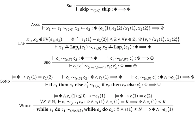
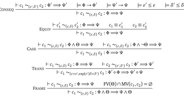
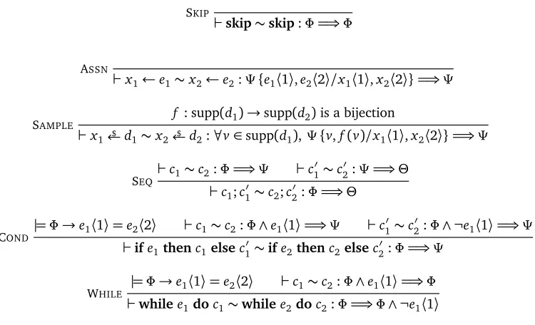
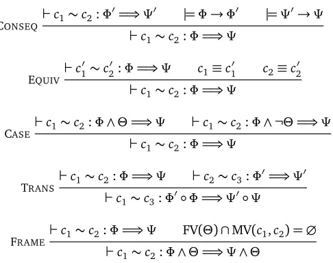
The rules ofPRHL can be divided into three groups: two-sidedrules,one-sidedrules, andstructural

rules. All judgments are parameterized by a logical contextρ, but since this context is assumed to be a fixed assignment of logical variables—constant throughout the proof—we omit it from the rules. The two-sided rules in Fig.2.2apply when the two programs in the conclusion judgment have the same top-level shape.

The rule[SAMPLE]is more subtle. In some ways it is the key rule inPRHL, allowing us to select a coupling for a pair of sampling instructions. To gain intuition, the following rule is a special case:

SAMPLE*

f : supp(d)_→supp(d)is a bijection

`x $

←d_∼x $

←d:>=⇒f(x_〈1〉) =x_〈2〉

The conclusion states that there exists a coupling of a distributiondwith itself such that each samplex

fromdis related to f(x). Soundness of this rule crucially relies ondbeinguniform—as we have seen, any bijection f induces a coupling of uniform distributions (cf. Example2.1.4). It is possible to support general distributions at the cost of a more complicated side-condition,2_{but we will not need this generality.} The full rule[SAMPLE]can prove a post-condition of any shape: a post-condition holds after sampling if it holds before sampling, wherex〈1〉andx〈2〉are replaced by any two coupled samples(v,f(v)).

The rule[SEQ]resembles the normal rule for sequential composition in Hoare logic, but its reading is more subtle. In particular, note that the intermediate assertionΨis interpreted differently in the two premises: in the first judgment it is a post-condition and interpreted as a relation betweendistributions over memoriesvia lifting, while in the second judgment it is a pre-condition and interpreted as a relation betweenmemories.

The next two rules deal with branching commands. Rule[COND]requires that the guardse₁〈1〉and

e₂〈2〉are equal assuming the pre-conditionΦ. The rule is otherwise similar to the standard Hoare logic rule: if we can prove the post-conditionΨwhen the guard is initially true and when the guard is initially false, then we can prove_Ψas a post-condition of the conditional.

Rule_[WHILE]uses a similar idea for loops. We again assume that the guards are initially equal, and we also assume that they are equal in the post-condition of the loop body. Since the judgments are interpreted in terms of couplings, this second condition is a bit subtle. For one thing, the rule does

notrequiree₁〈1〉=e₂〈2〉in all possible executions of the two programs—this would be a rather severe restriction, for instance ruling out programs wheree₁〈1〉ande₂〈2〉are probabilistic. Rather, the guards only need to be equalunder the coupling of the two programs given by the premise. The upshot is that by selecting appropriate couplings in the loop body, we can assume the guards are equal when analyzing loops with probabilistic guards. The rule is otherwise similar to the usual Hoare logic rule, whereΦis the loop invariant.

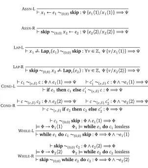
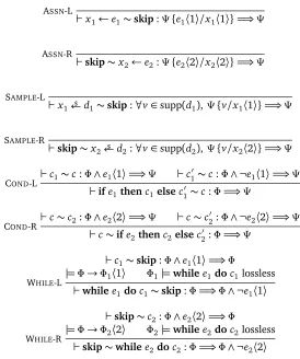
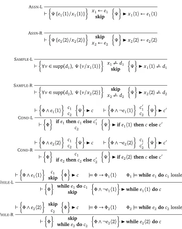
So far, we have seen rules that relate two programs of the same shape. These are the most commonly used rules inPRHL, as relational reasoning is most powerful when comparing two highly similar (or even the same) programs. However, in some cases we may need to reason about two programs with different shapes, even if the two top-level commands are the same. For instance, if we can’t guarantee two executions of a program follow the same path at a conditional statement under a coupling, we must relate the two different branches. For this kind of reasoning, we can fall back on theone-sidedrules in Fig.2.3. These rules relate a command of a particular shape withskipor an arbitrary command. Each rule comes in a left- and a right-side version.

The assignment rules,[ASSN-L]and[ASSN-R], relate an assignment instruction toskipusing the usual Hoare rule for assignment instructions. The sampling rules,[SAMPLE-L]and[SAMPLE-R], are similar; they relate a sampling instruction toskipif the post-condition holds for all possible values of the sample. These rules represent couplings where fresh randomness is used, i.e., where randomness is not shared between the two programs.

The conditional rules,[COND-L]and[COND-R], are similar to the two-sided conditional rule except there is no assumption of synchronized guards—the other commandcmight not even be a conditional. If we can relate the general commandcto the true branch when the guard is true and relatecto the false branch when the guard is false, then we can relatecto the whole conditional.

The rules for loops,_[WHILE-L]and[WHILE-R], can only relate loops to theskip; a loop that executes multiple iterations cannot be directly related to an arbitrary command that executes only once. These rules mimic the usual loop rule from Hoare logic, with a critical side-condition:losslessness.