The MapReduce‑based approach
to improve the shortest path computation
in large‑scale road networks: the case of A*
algorithm
Wilfried Yves Hamilton Adoni, Tarik Nahhal, Brahim Aghezzaf
*and Abdeltif Elbyed
Introduction
With the increasing size of road networks (4.4 billions of vertices and 6 billions of uploaded GPS points, according to OpenStreetMap data stats 2018 [1]), there has been vast improvement in hardware architecture for intelligent transportation system. The traditional GPS systems embedded in vehicles are only designed to find the shortest paths in small or medium road networks. With the increase in the size of road-networks, implementing efficient GPS programs has become challenging. This is mainly due to impractical computational time taken to compute the optimal path.
The basic algorithms used for the Single Source Shortest Path Problem (SSSPP) are not suited for intensive computation in large-scale networks because of long latency time. This is one of the crucial problem of route-guidance systems for highway vehicles including the Vehicle Routing Problem (VPR), Traveling Salesman Problem (TSP) and Pickup and Delivery Problem (PDP).
Currently, there are lot of approach of SSSPP such as label setting, dynamic pro-gramming, heuristic and/or bidirectional heuristic. However, they are inefficient
Abstract
This paper deals with an efficient parallel and distributed framework for intensive com-putation with A* algorithm based on MapReduce concept. The A* algorithm is one of the most popular graph traversal algorithm used in route guidance. It requires expo-nential time computation and very costly hardware to compute the shortest path on large-scale networks. Thus, it is necessary to reduce the time complexity while exploit-ing a low cost commodity hardwares. To cope with this situation, we propose a novel approach that reduces the A* algorithm into a set of Map and Reduce tasks for running the path computation on Hadoop MapReduce framework. An application on real road networks illustrates the feasibility and reliability of the proposed framework. The experi-ments performed on a 6-node Hadoop cluster proves that the proposed approach outperforms A* algorithm and achieves significant gain in terms of computation time. Keywords: Path-finding, Large-scale network, A* algorithm, Big Data, Hadoop,
MapReduce, HDFS, Parallel and distributed computing
Open Access
© The Author(s) 2018. This article is distributed under the terms of the Creative Commons Attribution 4.0 International License (http://creat iveco mmons .org/licen ses/by/4.0/), which permits unrestricted use, distribution, and reproduction in any medium, provided you give appropriate credit to the original author(s) and the source, provide a link to the Creative Commons license, and indicate if changes were made.
RESEARCH
when applied to NP-complete problems due to the large graph size, the hardware requirements and the time complexity. One of the problems emanating from the SSSPP is path finding in large road networks particularly with A* algorithm [2].
A* is mostly used in computer game and artificial intelligence. It is based on heu-ristic approach and presents great interest in the area of logistics/transportations, bioinformatics and social networks. The main problem is that A* is not adapted for intensive computation on large networks that consisting of millions of vertices and edges. It needs more resources in term of hardware configuration and the computa-tional time increases significantly when we encounter larger graph size. For example, it will be very difficult for car drivers who travels long distances to get high quality solution in order to take a right decisions in some cases where the quick response is a necessity.
In this context, several research studies have been carried out in order to improve the efficiency of graph traversal algorithms based on Big Data technology. This new technology has attracted the attention of business and academic communities (e.g. vehicle controls on big traffic events [3]) because of its ability to meet the 5V (Vol-ume, Velocity, Variety, Veracity and Value) challenges related to shortest path que-ries in large graphs. Most of the the efficient approaches [4–9] dedicated to these routing problems are based on the concept of parallel and distributed computing provided by Hadoop MapReduce [10].
We focus on an enhanced version of A* that runs in parallel and distributed envi-ronment with low cost commodity computers. Our objective is to define a high qual-ity path in reasonable computational time. This research work is inspired by papers [6, 7]. The key contributions of this paper are as follow:
• Firstly, we propose a MapReduce framework that promotes parallel and distrib-uted computing of shortest path in large-scale graph with A* algorithm.
• Secondly, our experimental analysis proves that the MapReduce version of A* outperforms the direct resolution approach of A*, and significantly reduce the time complexity with high quality results. In addition, our framework is reliable on real road network and works well with the scalability of network size.
• Finally, we show by comparison that the proposed MapReduce framework of A* algorithm is more effective than the MapReduce framework of Dijkstra algorithm presented in [6, 7].
Related work
Sequential shortest paths computing
For some time now, the shortest path problem has aroused more interest especially when applying it in the fields of transportation engineering and artificial intelligence. So several path-finding algorithms have emerged and there is a rich collection of literature in the current state of art [11–15]. The problem of concern is that SSSPP consists of find-ing the best path from an origin to a destination in graph.
Dijkstra [16] presented a Dijkstra’s algorithm for finding the shortest path from an origin-to-destination vertex in directed graphs with unbounded non-negative weights. Dijkstra’s algorithm works as breadth-first search [17]. It maintains a set of candidate vertices in a temporary queue and tends to expand the search space in all directions. Dijkstra’s algorithm is much faster than Bellman–Ford’s algorithm [15] and runs in O(n2)
[18–20] but is limited to smaller-scale graphs.
In another related work, Xu et al. [21] introduced a Fibonacci head [22] to improve the Dijkstra’s algorithm, this approach allowed to reduce the computational time to
O(m+nlog(n)) and is very practical to find the shortest path in graph containing large numbers of vertices. Orlin et al. [23] followed this work by integrating binary heaps to speed up the process of finding edges which minimizes the path length, their contribu-tion allowed to improve the time complexity to O(mlog(m)).
In another early contribution, Ira and Poh [24] proposed a bidirectional search method consisting of partitioning the global search domain under two and compute simultane-ously the path on the two sub-domains. This approach is inspiring but presents some limitations due to hardware requirements when the search domain became very large. Other classes of path-finding algorithms that use heuristic approaches aim to reduce the space domain and avoid unpromising vertices. Currently the best known shortest path approach that uses heuristic approach is A* algorithm [2].
Distributed shortest paths computing
When the data is too large, sequential algorithms became traditional and inefficient. In this sense, many related works have been performed to improve the velocity of exist-ing path-findexist-ing algorithms [4–9]. Presently, the most promising strategy for intensive path computation in large-scale graph is the parallel and distributed model. The use of this approach comes from the failure to handle big graph with traditional technique [25]. There have been a lot of studies on parallelizing the shortest path algorithms. Work con-ducted by Djidjev et al. [4] aims to improve by twofold the path computation in large graph with Floyd–Warshall algorithm. The authors proposed a parallel model of Floyd– Warshall based on Graphics Processing Unit (GPU).
Cohen and Jonathan [26] proved that the concept of distributed computing with MapReduce-based approach could be applied successfully in large-scale graph problems such as graph mining [5] and shortest path problem [6, 7].
experiments revealed that their approach reduces significantly the execution time and works well with the increasing number of cluster nodes (computers).
In recent papers [6, 7], the authors presented the MapReduce-based approach for shortest path problem in large-scale network. The proposed approach works in four stages including the map and reduce stages. Before the map stage, they had parti-tioned the graph into subgraphs and mapped them to each node. Next, Dijkstra’s pro-gram [16] is running on each machine to generate a set of intermediate paths. Finally in the reduce stage, all intermediate paths are aggregated to obtain the final shortest path. The authors contributions enabled a significant gain in terms of time complex-ity. In another work, Zhang and Xiong [8] followed the same approach for the search of dynamic path in large road network based on cloud computing. In addition, Seun-ghyeon et al. [27] proposed a parallel version of Girvan–Newman algorithm based on the concept of Hadoop MapReduce to improve the computational time in large-scale network.
Background
Hadoop and MapReduce
According to Hadoop documentation [10], Hadoop is an Apache open source frame-work inspired by Google File System [28]. It allows parallel processing on distributed data sets across a cluster of multiple nodes connected under a master-slaves architec-ture. Hadoop consists of two main components: HDFS [28] and MapReduce [29, 30].
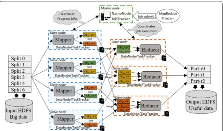
The first component is the Hadoop Distributed File System (HDFS). HDFS is designed to support very large file of data sets. It is also distributed, scalable and fault-tolerant. The Big Data file uploaded into the HDFS is split into block file with specific size defined by the client and replicated across the cluster nodes. The master node (NameNode) man-ages the distributed file system, namespace and metadata. While the slave nodes (Data-Node) manage the storage of block files and periodically report the status to NameNode. The second one is the MapReduce programming model for intensive computation on large data sets in parallel way. To ensure good parallelism, the data input/output needs to be uploaded into the HDFS. In MapReduce framework, the master node works as JobTracker and the slave nodes as TaskTracker. The JobTracker assumes the responsibil-ity and coordinates the job execution. The TaskTracker runs all tasks submitted by the JobTracker. As shown in Fig. 1, the MapReduce job runs in two main stages:
1 In the Map stage, the mappers (map tasks) are assigned to slave nodes that host the blocks data. Each mapper takes line-by-line the records of its input and transforms them into <key, value> pairs. Next, the map function defined by the user is called to produces another intermediate <key, value> pairs. The intermediate results are sorted locally by keys and sent to the reduce stage when all map tasks are completed. 2 In the Reduce stage, the reducers (reduce tasks) read the map stage outputs and
A* algorithm
A* or some extended version (HPA*, SMA*, MA* and IDA*) [14, 31, 32] of it, is one of the most used algorithm for SSSPP and was originally presented by Hart et al. [2] in 1986. It can be viewed as an extension of Dijkstra algorithm [16] by adding a heuristic function h that guides the search [11].
Suppose that a road network is denoted by a graph G= (V, E) where:
• V is the finite set of vertices of the graph G.
• E is the set of edges, such as: if (v,u)∈E , then there is an edge between the verti-ces v and u.
• We define the length function l:V ×V �→R+ , which for each edge (v, u), we associate a length l(v, u) if there is an edge between v and u, else ∞ if there is no edge.
• For each vertex v∈V , we define a distance d:V �→R+ such as d(v)= ∞ if we
can-not reach the goal vertex from v.
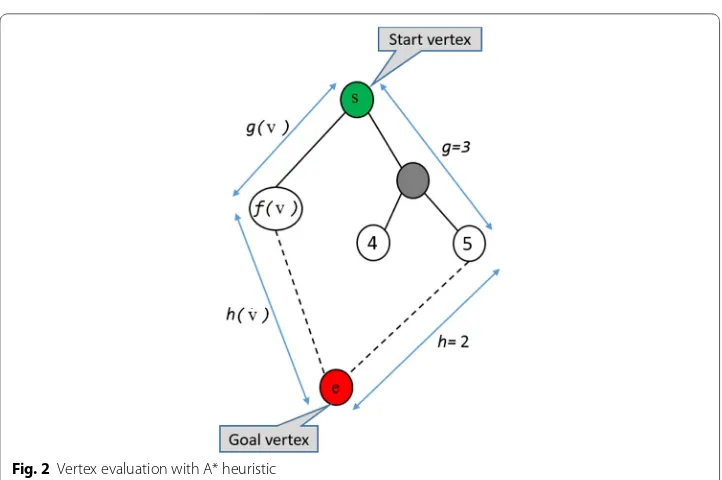
As shown in Fig. 2, A* takes advantage of heuristic function to avoid the exploration of unnecessary vertices that do not seem to be promising. A* incorporates an estimate of the path cost d(v) in which we can determine: (1) the costg(v) from the starting vertex s
to any vertex v∈V and (2) the rest of the ’path-completion’ h(v) from v to goal vertex e
[33].
The principle of path-finding with A* can be described as follows:
Step 1 initialization set O= ∅ and S= ∅;
begin by setting g(v)= ∞ for each vertex v∈V; next set current vertex c=s , g(s)=0 and d(s)=h(s);
finally set c=s and let S= {s};
Step 2 vertex expanding
for each vertex v∈V where edge (c,v)∈E ; if g(v) >g(c)+l(c,v) then update g(v)=g(c)+l(c,v) ; set d(v)=g(v)+h(v) , set d(v)=g(v)+h(v) and when v∈/O
let O=O+ {v};
Step 3 selection of promising vertex v∗
identify vertex v∗∈O where d(v∗)≤d(v) for all v∈O ; set O=O− {v∗} and S=S+ {v∗};
set c=v∗;
Step 4 stopping criteria
if c=e then the path has been found; elseif O= ∅ then failure;
otherwise go to step 2.
Like Dijkstra [16], A* works with two main queues: the ‘open-list’ O containing all candidate vertices and the ’close-list’ S that contains promising vertices. It applies a Depth-First-Search algorithm [34] to expand deeper-and-deeper all candidate verti-ces until the ’open-list’ is empty or until the goal vertex e is found. Then the search backtracks to explore in the most recent vertex v∈V−O that is not visited. To find
the most promising vertex v∗ , A* evaluates for each candidate vertex v∈O a tempo-rary distance d(v) such as d(v)=g(v)+h(v) . A* guarantees to find the optimal path if for every edge (v,u)∈E , h(v) verifies the triangle inequality: h(v)≤l(v,u)+h(v) and
h(e)=0 . Then for every vertex v∈V , the heuristic h(v) is said to be admissible.
Each time a new vertex is added in the priority queue, the ‘open-list’ needs to be sorted again and takes O(log(n)) time to complete all operations of enqueue and dequeue. For this reason, all vertices v∈O persist temporarily in memory. Hence, it can result in serious performance bottlenecks and runs very slowly because of expo-nential space memory consumption for infinity large number of vertices. In terms of the depth of the solution, A* runs in O(lb) time where l is the length of the shortest
path and b is the average number of successors per state. It is more logic to describe the time complexity taking account of vertices and edges of the graph, therefore it should be O((n+m)log(n)) . To improve the computation time in large graph, we assume that it’s necessary to:
1. Reduce the graph size by deleting some unnecessary vertices and edges of the graph; 2. Use sophisticated computers equipped with lot of ram memory for data persistence
or run A* with multitasks approach such as HPA* [32];
3. Use MapReduce approach to run the A* program under a distributed environment.
Reducing the graph size before applying A* search can take quite some time ( O(log(nb)) ) to perform the graph reconstruction after removing some unnecessary vertices. In some cases, there is a risk of removing some promising vertices that can affect the path opti-mality. Using powerful computers equipped with a lot of RAM memory and CPU power is another technique. However, difficulties arise when reaching hardware memory limits at a few million vertices. In this sense, the basic idea is to propose a parallel and distrib-uted version of A* based on MapReduce. Let’s see if the proposed approach is well suited to face the graph’s scalability in term of volume, the velocity in terms of time complexity and result quality in terms of veracity.
Proposed MapReduce version of A*
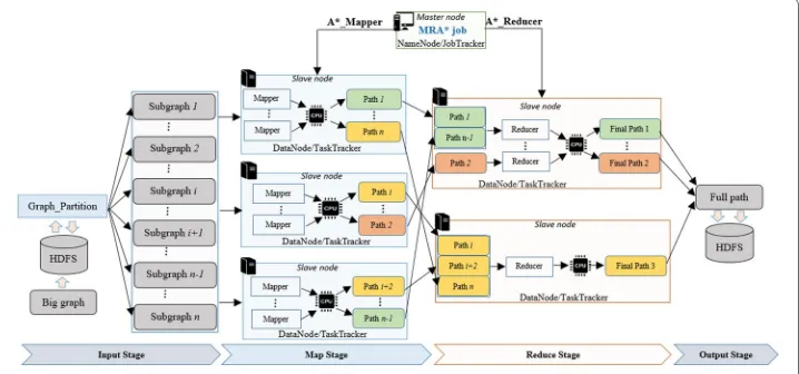
As shown in Fig. 3, the proposed MapReduce framework of A* (MRA*) is composed of four main stages:
1. Input stage: partition of the initial graph 2. Map stage: computation of intermediate paths 3. Reduce stage: concatenation of intermediate paths 4. Output stage: storage of full path
The MRA* job submitted from the master node is split into mappers and reducers that run respectively in the map and reduce stages. The set of stages are synchronized so that the output of the previous stage is chained to the input of the next stage. The
intermediate paths computing take place in the Map and Reduce stages. Consider that tmap and tred are respectively the time passed in the map and reduce stages, thus the total computation time TMRA∗ required by the MapReduce-A* framework to satisfy the full
path computation is calculated as follows:
Input stage: partition of the initial graph
The input stage (pre-processing stage) consists of uploading the initial graph data with specific size Gsize into the HDFS and partitioning it into set of subgraphs. By default, Hadoop splits physically the graph data into little files based on the defined block size Bsize and replicates them across the cluster nodes. Then the total number of block Nblock
occupied by the graph can be obtained using the following formula:
The graph partitioning is done by the Graph_Partition procedure (see Algorithm 1), it takes 3 parameters:
• l: subgraph length in km;
• A: source vertex;
• E: target vertex.
This procedure starts by computing the straight line distance L between the source vertex A and the target vertex E by using the Euclidean_Distance function (see Algo-rithm 2). Next, the obtained distance is divided by the diagonal length d in km to deter-mine the total number of subgraphs Ngraph using the following formula:
Each subgraph is delimited by its starting (C.lon, C.lat) and ending (D.lon, D.lat) posi-tions. The Subgraph_Position function (see Algorithm 3) is called to determine the GPS position of each subgraph. Next, we proceed to the creation of the subgraphs by invoking the Create_Subgraph function (see Algorithm 4). Finally, the set of vertices and edges of each generated subgraph is stored into the HDFS in form of key-value pairs as the Fig. 4 shows. It’s important to note that, the variation of the number of subgraphs
Ngraph relative to the number of block Nblock has an impact on the result quality,
espe-cially the path cost CMRA∗ . The optimality error ǫ between A* and MRA* is calculated as follows:
(1)
TMRA∗=tmap+tred
(2)
Nblock=E
Gsize
Bsize
+θ
whereθ =
0, if Gsize≡Bsize
1, else
(3)
Ngraph=L d
= L
l×√2
(4)
ǫ=CMRA∗−CA∗ CA∗ ×
Algorithm 2 describes the Euclidean_Distance function for computing the distance between two points of the graph. It takes as input the starting and ending vertices (points A and E) and applies the Euclidean formula [2] to determine the distance L.
Figure 5 illustrates a travel from Kingsport to Santa Rosa. The estimated travel dis-tance is given by the straight line (vector −AE→ ) based on the Euclidean_Distance
function. While, the projected line (arc AE ) passes through approximately Kingsport in north Carolina (point A), northeast of Missouri (point B), midwest of Nebraska (point C), northwest of Utah (point D) and Santa Rosa in California (point E). The application of Subgraph_Position function described in Algorithm 3 allows to split the projected line and calculates the ending position of each subgraph. It consists of four steps and takes four parameters:
• d: diagonal length in km;
• i: ith subgraph;
• (A.lon, A.lat): GPS coordinates of the source vertex (point A);
• (E.lon, E.lat): GPS coordinates of the target vertex (point E).
The first step (lines 11–12) consists of converting the GPS coordinates of the input points into cartesian coordinates. This step is necessary because it ensures high accuracy on large road network. In the second step (lines 14–16), we use the con-verted coordinates to calculate the normal vector (a, b, c) of the plane OAB (see Fig. 5a) assuming that O is the center of the earth with its cartesian coordinates (0, 0, 0). In the third step (lines 18–21), the obtained vector is used to determine the end-ing position of the ith subgraph. As shown in Fig. 5b, the point B is the ending point of the 1st subgraph, it partitions the projected arc ⌢
AE into vectors −AB→ and −BE→ . The
length of vector −AB→ is equal to d×i . Moreover, the length of vector −AE→ is equal to
r×α where r is the earth radius and α=(AO,−→−→OE) is the angle between −→AO and −→OE
(see Fig. 5a). Then we can deduce that the angle β=(−→AO,−→OB) between −→AO and −→OB
is equal to d×r×i [6]. The obtained angle β value is used to compute the cartesian
coordinates (B.x, B.y, B.z) of the point B by assuming that the unit of the normal vector (a, b, c) represents the rotation axis. The last step (line 23) is to convert back the cartesian coordinates of the point B into GPS coordinates (B.lon, B.lat) for carto-graphic projection.
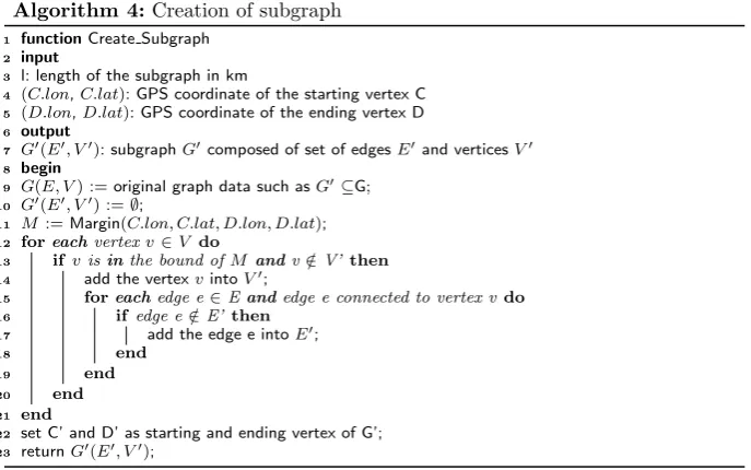
The Create_Subgraph function described in Algorithm 4, is called after finding the position of the subgraph. It takes as input the GPS coordinates of the position and length in km of the subgraph. Next, it builds from the original graph G(E, V) a new subgraph G′(E′,V′) where the positions of the vertices are into the boundary M
delimited by the starting (point C) and ending position (point D) of the subgraph.
Map stage: computation of intermediate paths
the used block size, then the total number of mapper Nmap is equal to the number of
block Nblock occupied by the initial graph, else the number of mapper used is equal to the number of subgraph Ngraph.
It is important to note that the velocity of all path computations depends on the number of cluster nodes Nnode and the number of core processors Ncoremap allocated per node. In
addition, the time complexity mi,j,k of the ith mapper assigned to the kth core of the jth
node is about O((n′+m′)log(n′)) where n′ is the number of vertices and m′ the
num-ber of edges of the ith subgraph. When one node finishes running its mappers, it waits until all other nodes complete their tasks before sending the results to the reduce stage. Therefore the total time tmap passed in the map stage is calculated as follows:
The A*_Mapper procedure described in Algorithm 5 takes the subgraph data as key-value pairs according to the structure of the vertices (see Fig. 4). The proposed algorithm is based on the classical version of A*. It consists of 3 steps. The first step (lines 9–15) is the initialization phase. The second step (lines 16–20) consists of exploring and selecting the most promising vertices until the target vertex found. This is achieved through the
Expand_Vertex and Select_Vertex functions. In the final step (lines 21–24), the Gen-erate_Path function is called for the extraction of the path from the selected vertices. Afterward, the result is stored locally until the other map tasks are completed before sending it to the reduce stage.
(5)
Nmap=
Nblock, if Bsize≤Gsize′ Ngraph, if Bsize>G′size
(6)
tmap=max
Nnode �
i=1 Nmap
�
j=1 N�coremap
k=1 mi,j,k
Algorithm 6 describes the Expand_Vertex function, it takes as input parameters the openlist O, the subgraph G′ and the current vertex c to expand. Next, it explores
in depth the neighborhood of the current vertex. For each expanded vertex, it evalu-ates the cost and verifies the triangle equality before adding it to the openlist.
Algorithm 7 describes the Select_Vertex function, it takes as input parameters the openlist O and the closelist S. It returns the most promising vertex v∗ where
d(v∗)≤d(v) for each vertex v in the openlist O.
Algorithm 8 describes the Generate_Path function, it takes as input the closelist S
Reduce stage: concatenation of intermediate paths
In the reduce stage, the set of intermediate paths from the map stage are concate-nated based on the path key. This is achieved by running the A*_Reducer (reducer) in parallel way. The total number of reducer Nred used to complete the reduce stage
depends on the number of nodes Nnode and the number of core processors Ncorered
allo-cated per node. The right number of reducers used to ensure good parallelism is cal-culated as follows [10]:
With 0.95, we assume that all nodes have the same hardware configurations (ram and cpu speed) and run averagely the same number of reduce tasks in the same gap of time. While with 1.75, the hardware configurations of the cluster nodes are different. The faster nodes will run more reduce tasks and lunch immediately another wave of reducers when they finish. So the total time tred passed in the reduce stage depends on the time ri,j,k of the ith reducer assigned to the kth core processor of the jth node. It’s calculated as follows:
The A*_Reducer procedure described in Algorithm 9 takes as input the array of inter-mediate paths which share the same path key and concatenates them. The ending extremity of the (i−1)th path becomes the starting extremity of the ith path so on until concatenation of the last path. Then the reducer waits until the other reducers complete its tasks before emitting the result to the master node.
Algorithm 9:Paths aggregating
1 procedureA* Reducer 2 input
3 [SP]: array of intermediate paths
4 output
5 F SP: the final shortest path 6 begin
7 F SP:= null;
8 foreachpathp∈SP.valuedo
9 F SP:= concat(F SP,p);
10 end
11 wait until all reduce tasks have been completed; 12 emit(key: pathId , val:F SP);
(7)
Nred=
0.95×Nnode×Ncorered 1.75×Nnode×Ncorered
(8)
tred=max
N�node
i=1 Nred � j=1 Nred core � k=1 ri,j,k
Output Stage: Storage of full path
In the last stage, the master node uploads the full path into the HDFS. Each path is writ-ten into a separate file. The full path is obtained by merging the conwrit-tent of the reduce files. To ensure fault tolerance, the cluster copies each file onto a separate peer node according to the replication factor.
Experimental results
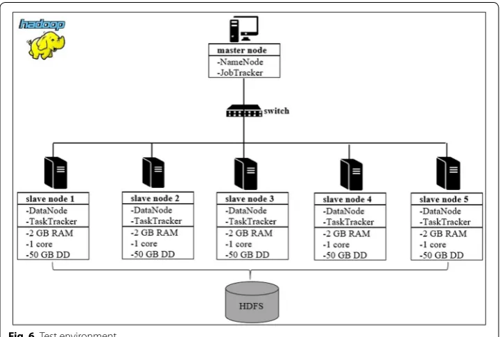
The performance tests were conducted on a 6-nodes Hadoop cluster. The configuration of the cluster is composed of 1 master node and 5 slave nodes as shown in Fig. 6. The nodes are connected through a local area network composed of a set of Ethernet cables Cat-5 100 Mbps that are directly plugged into a switch DES-1016D 100 Mbps. Each node within the cluster is equipped with a 4-core 2.3 GHz Intel i5 processor based on Linux SUSE-3.0.101 32 bit. The tests have been achieved on Hadoop 2.2.0. All computa-tions have been executed ten times and the presented values are the average values of the executions. Table 1 presents all set of parameters of our experiment.
Fig. 6 Test environment
Table 1 Experimental parameter set
Parameter type Parameter designation Parameter value
Nnode No. of cluster nodes 6
n No. of graph vertices [8000, 100,000]
Gsize Graph size in Gbit [0.2, 16.6]
Bsize Block size in Mbit {64, 128, 256}
G′
size Subgraph size in Gbit [0.3, 2]
l Subgraph length in km [20, 400]
Ncoremap No. of map cores {1, 2, 3, 4}
Data set
The real-world road data used are benchmark data gathered from OpenStreetMap (OSM) spatial database [35]. The data are stored in the .osm.pbf data format, an alterna-tive to XML based formats (KML and GML). The XML file contains points, ways, rela-tions and nested tags in each of these objects. The graph data covers all types of road networks, including local roads, and contains weighted edges to estimate the travel dis-tances/times. We used QGIS Desktop 2.18.3 and JOSM’s (Java OpenStreetMap Editor) tool to extract information. The criteria of filtering is based on ’osm_tab’, we extracted all objects whose tag keys corresponds to ’highway’.
Application: road trip from northern to southern Morocco
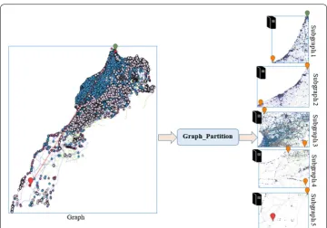
This section presents a case of application of the proposed framework on Moroccan road network in order to find the shortest path from Tangier (northern Morocco) to Dahkla (southern Morocco). It is the equivalent of nearly 1800 km of road trip. The extracted graph consists of 726,467 vertices. Firstly, the road network is split into five subgraphs as shown in Fig. 7. Each partition is assigned to one node of the cluster and is delimited by its starting point and ending point (see Table 2). Secondly, the compu-tation of the intermediate paths is carried out in parallel way across the cluster node, as shown in Fig. 8. We get 5 paths, each path represents a partial solution. Next, the full path is obtained by merging several times all partial solutions (see Fig. 9). Finally, the full solution is written into the HDFS and each part of the solution is written in separated files as shown in Fig. 10.
Ratio of MapReduce‑A* efficiency versus direct resolution
To prove the efficiency of the proposed framework, we performed tests with different road graphs on a single-node cluster. This means that only one node plays both the master and slave roles. Table 3 reports the computational times between A* and our MRA*. Columns TA∗ and TMRA∗ contain respectively the computation times in sec-onds of A* and MRA∗ . We remarked that the proposed version of A* outperformed
the sequential A* and it reduces considerably the time complexity. For example with a graph size of 7 Gbit composed of 70,000 vertices and 3.6 billion of data recording in its adjacent matrix, we computed the shortest path in 2939 s (00:26:40) with our
MRA∗ approach versus 177,948 s (49:25:48 ≈ 2 days 27 min) with A∗ . In many worst cases, we had to kill and rerun the execution of the sequential A* program when we faced problem with Java heap memory. The improvement ratio shows that the pro-posed approach is on average 150 times faster than sequential A*. By deduction we noted that MRA∗ is also 15 times faster than HPA* (another extension of A*), given that it has been shown in [31] that HPA* is on average ten times faster than A*.
Influence of number of core processors on the computational time
The first topic of interest consists of analyzing the impact of increasing number of core processors per node on the computational time. Figure 11 shows that the increasing number of cores reduces the total computational time. Whenever a new core processor Table 2 Subgraph boundaries
Subgraph Starting point Ending point
Name Lat lon Name Lat lon
1 Tangier 35.759 − 5.818 El Gara 33.24 − 7.15
2 El Gara 33.24 − 7.15 Ait M’Hamed 31.857 − 6.498
3 Ait M’Hamed 31.857 − 6.498 Ikiafene 29.663 − 9.638
4 Ikiafene 29.663 − 9.638 Boukraa 26.341 − 12.841
5 Boukraa 26.341 − 12.841 Dahkla 23.03 − 15.02
Fig. 9 Reduce stage: concatenation of partial paths. The set of intermediate paths are merged to build the full path
is used, the computational time is improved considerably, in particular the time of the map stage. We also remarked that the map time occupies on average 90% of total time. This is explained by the fact that the tasks in the map stage run on all the vertices of the graph, unlike the reduce stage where the tasks run on the selected vertices (vertices in
closelist).
Influence of number of Hadoop nodes on the computational time
The second topic of interest is the impact of the increasing cluster nodes on the com-putational time. We performed a tests with a graphs size ranging from 103 Mbit to 16.6 Gbit. Figure 12 shows the influence of the number of slave nodes on the com-putational time. We remarked that the comcom-putational time varies strongly and is significantly improved when extending the cluster from 1 to 6 nodes. The addition of new nodes promote the decreasing of the exponential time complexity until the Table 3 Comparison of computational time in seconds time between A∗ and MRA∗
into a 1-node cluster
n No. data Gsize Time with A* Time with MRA* Ratio
TA∗ tmap tred TMRA∗ TA∗
TMRA∗
8000 64 × 106 0.25 1,5752 157 11 168 94
15,000 22.5 × 10⁷ 0.5 35,331 183 18 201 159
20,000 40 × 107 0.8 51,469 233 36 269 191
25,000 62.5 × 10⁷ 1.2 77,378 330 53 366 211
30,000 90 × 107 2 101,909 405 76 481 212
40,000 16 × 108 3 129,343 698 91 789 164
50,000 25 × 108 5 152,863 1035 103 1137 134
60,000 36 × 108 7 177,948 1397 203 1600 111
80,000 64 × 108 11.5 269,102 1790 408 2198 122
90,000 81 × 108 14 31,4425 2100 568 2668 118
100,000 10 × 109 16.6 359,747 2257 682 2939 122
Average ratio of time improvement 149
linearity time is reached. For example, with the same graph of 60,000 vertices, the time decreases from 1600 to 764 s with 2 nodes and from 764 to 322 s with 3 nodes. Beyond 3 nodes, the addition of new nodes does not improve the computational time. This means that the nodes 4, 5 and 6 are not used by the framework for the path com-putation. This leads us to consider that there exists an optimal number of nodes for a given graph that satisfies the full path computation.
Influence of number of subgraphs on the computational time and the result quality
The third topic of interest concerns the impact of number of subgraphs size on the com-putational time and the result quality. We performed the tests on a graph size of 1.6 Gbit containing 25,000 vertices. We physically split the graph under 9 blocks ( Nblock =9 )
while varying the total number of subgraphs from 1 to 16 ( Ngraph∈ [1, 16] ). The results in Fig. 13 show that when the number of subgraphs is lower than the number of blocks ( Ngraph<Nblock ), then the obtained result is optimal ( ǫ =0 ). On the other hand, when the number of subgraphs is greater than the number of blocks ( Ngraph>Nblock ), then the time is improved but to the detriment of the result quality (e.g. ǫ∈]0, 0.5%[ ). The best time that guarantees optimal results is obtained when the number of subgraphs is equal to the number of blocks ( Ngraph=Nblock =9).
Influence of blocks size and subgraphs length on the computational time
This topic of interest concerns the impact of blocks size variation on the computational time. We performed different tests by physically splitting the graph under blocks size
Bblock∈ {64, 128, 256}Mbit while varying the subgraphs length l from 40 to 400 km
(this corresponds respectively to a subgraphs size ranging from 0.34 to 2 Gbit). Table 4
reports the obtained results. We remarked that the computation time is faster with small blocks size (e.g. Bblock =64 Mbit). Also, this time increases with the increasing subgraphs length. Thirdly, when the subgraphs size is equal to or larger than the blocks size ( Gsize′ ≥Bsize ), the time does not improve and remains constant. For example with
the blocks size fixed to 64 Mbit, the time remains equal to 460 s for all subgraphs size
Gsize′ ≥64.
MapReduce‑A* versus MapReduce‑Dijkstra
In this section, we compare our framework with the MapReduce framework of Dijk-stra proposed by Aridhi et al. in [6]. We performed tests with the data sets of the french road network graph used in [6]. Figure 14 compares the computation time of our MapReduce-A* approach with the computation time of MapReduce-Dijkstra approach while ranging the subgraphs length l from 15 to 200 km. The test was also performed by varying the cluster size from 1 to 6 nodes. As shown in Fig. 14, we remarked that the two frameworks run more quickly in large cluster nodes and in all cases, they only use 4 nodes of the cluster to satisfy the shortest path computation. However the computation times differ according to the variation of the subgraphs length l in km. In the first two cases, when the subgraphs length are small (l= 15 km
Fig. 13 Impact of number of subgraphs on the computational time and the result quality
Table 4 Impact of blocks size and subgraphs length on the computational time in seconds
l G′
size Total time TMRA∗
Bsize=64 Bsize=128 Bsize=256
60 0.3 371 376 368
78 0.4 412 409 409
100 0.5 463 464 464
109 0.6 460 517 532
125 0.7 458 596 605
156 0.8 459 753 754
200 1 461 1003 1065
265 1.3 460 1008 1149
400 2 461 1004 1164
and l= 50 km), we remarked that the proposed framework is faster than MapReduce-Dijkstra framework. On the other hand, in the last two cases with large subgraphs (l = 100 km and l= 200 km), the MapReduce-Dijkstra framework presents better time
performance. Like the MapReduce-Dijkstra, the proposed MapReduce-A* frame-work consumes low number of machines in the cluster and is on average 1.15 time faster than MapReduce-Dijkstra. Moreover, our framework computes the full path in only one iteration instead of MapReduce framework of Dijkstra that requires many iterations.
Discussion
In this section, we are discussing about two topics related to the experiment results. The first topic concerns the optimal usage of the cluster. A cluster is defined as optimal if all nodes within the cluster participate in the full path computation. The answer to this question depends on the cluster configuration and the number of generated subgraphs. For the moment there is no formula for determining the optimal number of nodes for a given graph. However, a solution emanating from our experimental study consists of firstly splitting the graph under Nnode×Ncoremap subgraphs in the input stage. Secondly,
in the map stage we set the number of mappers to be equal to the number of subgraphs
( Nmap= Ngraph ). Third, in the reduce stage, we fix the number of reducers to Nnode×
Ncorered . This solution allows an optimal usage of the cluster but does not guarantee the
optimal solution.
The second topic treats the optimality of the obtained solution. As shown in the exper-imental analysis, the quality of results depends on two parameters: the subgraphs length in km and the blocks size. We have remarked that when we set the subgraphs length l so that the subgraphs size Gsize′ are on average equal to the blocks size Bsize , then we get a result without optimality error ( ǫ= 0). So to conclude, the optimal solution is obtained when G′size≈Bsize.
Conclusion and further works
To sum up, in this paper, we proposed a novel parallel and distributed version of A* for computing the shortest path in large-scale road networks. The proposed approach is based on MapReduce framework. The experiments demonstrated that our framework presents better performance and reduces significantly the computation time, it is scal-able and works well in large cluster. In addition to that, it is reliscal-able and can be used in GPS systems for navigating on very large road networks. In the light of all these, our work represents a contribution and may attract more interest for other graph traversal algorithms. It can be adapted and extended to social network analysis (e.g Facebook or Twitter) or DNA sequencing problem related to bioinformatic in order to accelerate the process of determining the order of nucleotides within DNA graph. For future work, we are interested in :
• Adapting the traveling salesman problem to such framework.
• Proposing a novel framework based on Big Data graph analysis tools such as Neo4j or Apache Shindig to better explore the road network graph.
Authors’ contributions
All mentioned authors contribute in the elaboration of the article. All authors read and approved the finalmanuscript.
Authors’ information
Wilfried Yves Hamilton Adoni received the B.S. degree in Computer Science from Hassan II University of Casablanca, Morocco in 2012. He received the M.E. degree in Operational Research and System Optimization from Hassan II Univer-sity of Casablanca, Morocco in 2014. He is currently in the final step of its Ph.D. in Computer Science, especially in Big Data technology and smart transportation with the Science Faculty, Hassan University of Casablanca, Morocco. He is currently Temporary Assistant, Teaching and Research, part time at Central School of Casablanca, Morocco. His research interests include Big Data, Graph Database, smart transportation, path-finding algorithm and traffic flow analysis. He joined the elite group of young Big Data Specialist with IBM BigInsights V2.1 in 2015. Wilfried Adoni can be contacted at: [email protected]/[email protected].
Tarik Nahhal is an Associate Professor of Computer Science in the Faculty of Science at Hassan II University of Casa-blanca. He holds a PhD in Hybrid System and Artificial Intelligence from the Joseph Fourier University, Grenoble I, France. His research interests include Hybrid System, Cloud Computing, Big Data, NoSQL Database, IoT and Artificial Intelligence. He has animated several Big Data conferences and has published several research articles in peer-reviewed international journals and conferences. He is Big Data specialist with IBM Big Data certification. His current research interests focus on high problem related to Big Data complexity. Dr Tarik Nahhal can be contacted at: [email protected].
Brahim Aghezzaf is a Full Professor of Operational Research at Hassan II University of Casablanca. His research inter-ests include optimization, logistics, transportation modeling, multiobjective optimization, heuristics and combinatorial optimization. Dr Brahim Aghezzaf has published several research articles in peer-reviewed international journals and conferences. He served several conferences as a program chair and program committee member for many international conferences. He has made several contributions in optimization problems. He holds Big Data certification by IBM and numerous scientific prices in the field of logistics/transportation optimization. Dr Brahim Aghezzaf is the corresponding author and can be contacted at: [email protected].
Abdeltif Elbyed is an Associate professor of Computer Science at Hassan II University of Casablanca. His research interests include E-learning, Interoperability, Ontologies, Semantic web, Multi-agent system and urban transportation. He has published several research papers. He is also Business Intelligence Specialist. His current research interests reverse logistics and urban mobility. Dr Abdeltif Elbyed can be contacted at: [email protected].
Acknowledgements Not applicable.
Competing interests
The authors declare that they have no competing interests.
Availability of data and materials
All supporting data files are open source. Map data used are available and can be accessed directly fromOpenStreetMap at http://downl oad.geofa brik.de and informations about the subgraph format of the extracted roadnetworks are avail-able at http://fc.isima.fr/˜lacomme/OR hadoop/.
Consent for publication Not applicable.
Funding Not applicable.
Publisher’s Note
Springer Nature remains neutral with regard to jurisdictional claims in published maps and institutional affiliations.
Received: 9 February 2018 Accepted: 20 April 2018
References
1. OpenStreetMap. OpenStreetMap statistics. https ://www.opens treet map.org/stats /data_stats .html. Accessed 19 Mar 2018.
2. Hart PE, Nilsson NJ, Raphael B. A formal basis for the heuristic determination of minimum cost paths. IEEE Trans Syst Sci Cybern. 1968;4(2):100–7.
3. Adoni WYH, Nahhal T, Aghezzaf B, Elbyed A. The mapreduce-based approach to improve vehicle controls on big traffic events. In: 2017 International colloquium on logistics and supply chain management (LOGISTIQUA). Rabat: IEEE; 2017. p. 1– 6. https ://doi.org/10.1109/LOGIS TIQUA .2017.79628 64.
4. Djidjev H, Chapuis G, Andonov R, Thulasidasan S, Lavenier D. All-pairs shortest path algorithms for planar graph for gpu-accelerated clusters. J Parallel Distrib Comput. 2015;85(C):91–103.
5. Aridhi S, d’Orazio L, Maddouri M, Mephu NE. Density-based data partitioning strategy to approximate large-scale subgraph mining. Inf Syst. 2015;48(Supplement C):213–23.
6. Aridhi S, Lacomme P, Benjamin V. A mapreduce-based approach for shortest path problem in large-scale networks. Eng Appl Artif Intell. 2015;41(C):151–65.
7. Aridhi S, Benjamin V, Lacomme P, Ren L. Shortest path resolution using hadoop. In: MOSIM 2014, 10ème Confèrence Francophone de Modèlisation, Optimisation et Simulation, Nancy, France; 2014.
8. Zhang D, Xiong L. The research of dynamic shortest path based on cloud computing. In: 2016 12th international conference on computational intelligence and security (CIS). Wuxi: IEEE; 2016. p. 452–455.
9. Plimpton SJ, Devine KD. Mapreduce in mpi for large-scale graph algorithms. Parallel Comput. 2011;37(9):610–32. 10. Hadoop, A. Welcome to Apache Hadoop. http://hadoo p.apach e.org/. Accessed 10 Mar 2017.
11. Cherkassky BV, Goldberg AV, Radzik T. Shortest paths algorithms: theory and experimental evaluation. Math Pro-gram. 1993;73:129–74.
12. Fu L, Sun D, Rilett LR. Heuristic shortest path algorithms for transportation applications: state of the art. Comput Oper Res. 2006;33(11):3324–43.
13. Schrijver A. On the history of the shortest path problem. Documenta Math ismp. 2012;17:155–67.
14. Goldberg AV, Harrelson C. Computing the shortest path: a search meets graph theory. In: Proceedings of the sixteenth annual ACM-SIAM symposium on discrete algorithms. Philadelphia: Society for Industrial and Applied Mathematics; 2005. p. 156–165.
15. Bellman R. On a routing problem. Quart Appl Math. 1958;16(1):87–90.
16. Dijkstra EW. A note on two problems in connexion with graphs. Numer math. 1959;1(1):269–71. 17. Zhou R, Hansen EA. Breadth-first heuristic search. Artif Intell. 2006;170(4):385–408.
18. Cormen TH, Leiserson CE, Rivest RL, Stein C. Introduction to algorithms. 2nd ed. Cambridge: MIT Press; 2001. 19. Skiena SS. The algorithm design manual. 2nd ed. London: Springer; 2008.
20. Even S. Graph algorithms. 2nd ed. New York: Cambridge University Press; 2011.
21. Xu MH, Liu YQ, Huang QL, Zhang YX, Luan GF. An improved dijkstra’s shortest path algorithm for sparse network. Appl Math Comput. 2007;185(1):247–54.
22. Fredman ML, Tarjan RE. Fibonacci heaps and their uses in improved network optimization algorithms. J ACM JACM. 1987;34(3):596–615.
23. Orlin JB, Madduri K, Subramani K, Williamson M. A faster algorithm for the single source shortest path problem with few distinct positive lengths. J Discrete Algorithms. 2010;8(2):189–98.
24. Ira P. Bi-directional search. Mach Intell. 1971;6:127–40.
25. Inokuchi A, Washio T, Motoda H. An apriori-based algorithm for mining frequent substructures from graph data. In: European conference on principles of data mining and knowledge discovery. Prague: Springer; 2000. p. 13– 23. 26. Cohen J. Graph twiddling in a MapReduce world. Comput Sci Eng. 2009;11(4):29–41.
27. Moon S, Lee JG, Kang M, Choy M, Lee JW. Parallel community detection on large graphs with MapReduce and GraphChi. Data Knowl Eng. 2016;104(Supplement C):17–31.
28. Ghemawat S, Gobioff H, Leung ST. The google file system. In: ACM SIGOPS operating systems review, vol. 37. New York: ACM; 2003. p. 29–43. https ://doi.org/10.1145/94544 5.94545 0.
29. Dean J, Ghemawat S. Mapreduce: simplified data processing on large clusters. Commun ACM. 2008;51(1):107–13. 30. Vavilapalli VK, Seth S, Saha B, Curino C, O’Malley O, Radia S, Reed B, Baldeschwieler E, Murthy AC, Douglas C, Agarwal
S, Konar M, Evans R, Graves T, Lowe J, Shah H. Apache hadoop YARN: yet another resource negotiator. In: Proceed-ings of the 4th annual symposium on cloud computing. Santa Clara: ACM Press; 2013. p. 1– 16.
31. Botea A, Müller M, Schaeffer J. Near optimal hierarchical path-finding. J Game Dev. 2004;1(1):7–28.
32. Russell S. Efficient memory-bounded search methods. In: Proceedings of the 10th European conference on artificial intelligence. New York: John Wiley & Sons; 1992. p. 1– 5.
33. Zeng W, Church RL. Finding shortest paths on real road networks: the case for a*. Int J Geogr Inf Sci. 2009;23(4):531–43.
34. Tarjan R. Depth-first search and linear graph algorithms. SIAM J Comput. 1972;1(2):146–60.