A method of designing a generic actor
model for a professional social network
Swapnil S Ninawe and Pallapa Venkataram
*Background
With the development of internet technology, a social network [1–4] provides a new way of communication, entertainment and gaining information [5]. Social networks [6–9] have influenced people of different regions and professionals to share the information due to the advancement in the technology [10, 11]. The main goal of a social network is to make the information space [12, 13] where a person can share information like thoughts, personal data, events, etc. It shares the basic purpose of interaction and com-munication [14], and specifies goals and patterns that vary significantly across different regions of people. Visibility of information [15, 16], structural variations [17, 18] and access [19–22] are the significant characteristics of a social network.
A social network is a social structure [23–27] among individuals known as actors or organisations. The social network also defines a group of actors connected by a set of relationships that are continuously changing. The crucial factor here is relationships among actors that are required for construction of a social network [28]. Hence, as an important research area, developing a social network focuses relationships associated
Abstract
The emergence of social networks have opened a new paradigm for professional groups to student groups to exchange their information with their contemporaries quickly and efficiently. The social networking enables to set up relations among the people (called actors) who share common interests, activities or connections. An actor or a person plays a predominant role in sharing social networking services, hence optimal modelling of an actor is essential. An actor model must be defined with several issues concerning to interests, activities, devices used, etc. In this paper, we present a generic actor model for a professional social network (GAMPSON) by considering actor’s personally identifiable information, professional information, activity, social status, etc. The designed GAMPSON is tested over professional social networks such as agriculture social network and museum social network, where GAMPSON generates unique actors associated with the agriculture and museum social network, and renders relations among the actors. Results demonstrated that it is simple and accurate to gen-erate actors and their relations in any social network along with provision of informa-tion over database.
Keywords: Generic actor model, Actor relation, Agriculture social network, Museum social network
Open Access
© 2015 Ninawe and Venkataram. This article is distributed under the terms of the Creative Commons Attribution 4.0 Interna-tional License (http://creativecommons.org/licenses/by/4.0/), which permits unrestricted use, distribution, and reproduction in any medium, provided you give appropriate credit to the original author(s) and the source, provide a link to the Creative Commons license, and indicate if changes were made.
RESEARCH
with the actors. Once a social network is constructed, it could be used to analyse knowl-edge discovery, finding access, searching actors, groups, relations, etc. In general, devel-oping a social network [29] covers the area of any network, and metrics used are based on the mathematics of graph theory [30–32] regardless of the connections. After con-structing a social network, its ultimate goal is sharing knowledge [33–36]. In summary, a social network consists of an actor, and its relevant information and association. Thus, an actor model in a social network is essential in precisely determining relation among the actors.
Social networks have gained importance for their functionality enabling people to obtain information based on relationships. This capability comes from a well-defined actor model. Therefore, first thing to architect should be the actor model by which rela-tionships can be build among actors. Formally modelling and analysing an actor model [37] for a social network has deep impact on the development of high quality social net-work systems. An actor model can have explicit form, meaning that we can determine specific things about an actor model. For example, relations among actors in a social network must be deterministic in nature, meaning that given a set of actors with defini-tive properties, a model should be able to replicate same relations every time. If an actor model is a good approximation of the real world social network actors, then a definitive assurance about the actor model gives us confidence in the real world realisation. Such certainty is crucial, particularly for social networks, where relation among actors are of utmost importance. A rigorous approach towards formalising and analysing the actor model can help us in determining relations among actors more effectively and efficiently. Studying actor models gives us insight into how social networks are helpful in the real world.
An actor model based on actor’s professional information, activity, etc., is difficult to address, and also dynamic data variations, changing relations and varying privileges imposes complexities in actor modelling. The social network simplifies the complexities, and there are few actor models that are currently deployed [37–39] which partially cov-ered professional information, activity, etc. in social networks.
Proposed idea
Organisation of the paper
The organisation of the rest of the paper is as follows. “Some of the existing actor mod-els of social networks” covers some of the existing actor modmod-els for social networks where we discussed different actors models that were built along with their advantages and disadvantages. Design of a GAMPSON was presented in “Generic actor model for a professional social network” along with distinct characteristic features of actors such as personal information, activity, etc. In order to demonstrate the applicability of the model, we designed the actor specifications from the generic model for the professional social networks such as agriculture social network (ASN) and museum social network (MSN) were given in “Design of an actor for the agriculture social network andmuseum social network using the GAMPSON” for provision of information such as seed, soil, crop, etc. to the actors in case of ASN and exhibit information in case of MSN, respec-tively. Simulation environment of ASN and MSN with the designed actors and testing results were discussed in “Simulation environment” and “Simulation results”, respec-tively. We compared the GAMPSON with other models, and showed results for accu-racy of the model and relation among the actors in case of ASN and MSN. At last, we concluded our work in “Conclusions”.
Some of the existing actor models of social networks
Some of the works on actor model were based on actor profile data, graph structures, connectivity relations, etc. Stochastic actor-based models for dynamics of directed net-works were studied [38] and showed an extended form can be used to analyse longitudi-nal data on social networks with changing attributes of the actors. The model supposed to use minimum mathematics along with some of the properties of graphs such as out-degree, reciprocity, ego, alter,etc., and used directed relations overall, but again did not consider basic properties of actors. In another work, Sudhakara [44] showed how vari-ous actors of energy system were making the system worked, and what incentives and constraints each of the actors experienced. This work was more related to household energy consumption and defined energy related actors based on their use. Use of profile data to construct a graph structure was carried out [39] and proposed a simple model to utilise both observable connectivity relation and profile graph. Here, much more rigor-ous mathematics was used along with similarity measures, and also specified weighted graph model to find relations among the actors. The main disadvantage with this model was its complexity in determining relations. Semantic annotation of abstract models of actor ecosystem [45] could be used to derive executable process models that realise those systems. Here, a partial actor eco system for a transport organisation was pro-posed with logical operators such as AND, OR and XOR. The advantage of this model was its simplicity in nature but lacked in precision. Other approach in building formal model of social network with rigorous maths along with algorithm were also studied in [46] illustrated the idea and demonstrated the effectiveness of high level Petri nets with channels for formally modelling of social networks and analysed a friend suggestion function in it. Again the disadvantage of such model was its complexity and understand-ability. In another approach, social relation extraction system using dependency-kernel-based support vector machine was proposed [47], and classified input sentences on the basis of describing social relations between two people. The social relation extraction process was too complex in nature and its applicability was limited.
We have made an attempt to capture the generic model of an actor of a specific pro-fessional social network. We have found that our model is complete by drawing a set of characteristic features of an actor based on the type of activities, social status, qualifica-tions, etc. rather than using tag or rule based approach. We also found that an actor can be defined by a set of generic features is more adaptable than using tags or rule based approaches. Our model is simple in nature and its applicability on social networks has produced good results.
Generic actor model for a professional social network
In this section, we present a GAMPSON which initially gathers distinct characteristic features of an actor such as personally identifiable information, professional information, social status, activity, and history (shown in Fig. 1). Depending upon an individual actor these characteristic features vary, and relations among actors can be built based on these characteristics features of the actors. Dynamic change of the characteristic features and varying relations among actors are the key factors in the proposed GAMPSON.
We define the actor of a social network as a five tuple and its structure is as follows.
(1)
ai=
PerIi,ProfIi,Acti,Histi,SocSi
where,
– Personally identifiable Information (PerIi) of the actor ai : PerIi is used to identify the
actor uniquely. We consider this information as PerIi= {peri1,per
2
i, ...,perin}. For
exam-ple, peri1=Name, peri2=address, peri3=IP address, per4i =Telephone number,
etc.
– Professional Information (ProIi) of the actor ai : ProIi is used to provide profession
information of the actor. We recognise this information as ProIi= {pro1i,pro
2
i, ...,promi }.
For example, pro1i =education, pro2i =occupation, pro3i =qualification, pro4i =role,
etc.
– Activity (Acti) of the actor ai : Acti is used to provide activity information of the
actor. We recognise this information as Acti= {acti1,acti2, ...,actip}. For example,
acti1=research, acti2=publications, etc.
– History (Histi) of the actor ai : Histi is used to indicate history of the actor. We consider
this information as Histi= {histi1,hist
2
i, ...,histis}. For example, hist
1
i =coordination, histi2=interactions, etc.
– Social Status (SocSi) of the actor ai : SocSi is used to indicate social information of
the actor. We consider this information as SocSi= {soc1i,soc
2
i, ...,socli}. For example,
soc1i =religion, soci2=ethnicity, soci3=class, soc4i =position, etc.
– Thus a typical actor ai in a social network can be represented as
Weight allocation to the actor’s characteristic features
We have considered values (see Table 1) for every characteristic feature to capture the realistic feature of an actor. In education system, if a person is BE (Bachelor of Engineer-ing), then he has supposed to pass 1st to 10th standard, then 2 years in junior college, and later 4 years in Engineering. Hence for BE we have taken 10 + 2 + 4 = 16. Similarly for BS it is 10 + 2 + 3 = 15 and for MS it is 10 + 2 + 3(for BS) + 2(for MS) = 17. For ME it is 10 + 2 + 4 + 2 = 18 and for PhD it is 10 + 2 + 4 + 2 + 5 = 23. We also have con-sidered type of work done by actors, class of degree, g-index and h-index for education. Hence the total weight of the actor ai based on education is calculated as
ai = {XYZ, 21st street(NY), 080−86945668,PhD,
For occupation, we have assigned exponential weights because the probability of occur-ring of an event or activity of an administrator is greater than banker, finance, and busi-nessman. For example, in the agriculture social network, the probability of a scientist (who is administrator) enquiring about soil contents, type of crop, etc. is greater than banker, farmer, and labourer. Also, a professor working in an engineering department will be less interested in the agriculture related activities than a professor in the depart-ment of organic chemistry. For history, since history always gets accumulated, hence the Gaussian curve will be formed due to law of large numbers. Consider actors ai and aj where if education level of ai is PhD then it takes value as 23, and education level of aj is ME then it takes value 18. Also, if an actor ai has name “Peter Allen” and an actor aj has name “John Allen”, then actors ai and aj have common sirname. Hence, the value of the name is given as 1 and same follows for home address, IP address, and telephone num-ber. Activity such as teaching, research activity, session, seminar, publications, research, conference attended, and positions held are assigned weights based on their rank. For example, if number of courses taught are two, then weight of teaching is 2.
Weight of education of ai =(Number of years spent the college by ai) +(g−index of ai)+(h−index of ai) +(class of degree of ai)
Table 1 Characteristic features and their values used in the GAMPSON
Characteristic features Sub characteristics Set Weights
1. Personally identifiable
information (PerI) Name (per 1
i) {Name of the actors} 1 for common name
Address (per2
i) {Home address of the
actors} 1 for common address
IP address (per3
i) {0.0.0.0.0.0 to FF.FF.FF.FF.
FF.FF} 1 for common IP address
Telephone number (per4
i) {Telephone numbers of this
actors} 1 for common tel-ephone number 2. Professional Information
(ProI) Education (pro
1
i) {PhD, ME, MS, BE, BS} 15I(BS)+16I(BE) +17I(MS)+18I(ME)
+23I(PhD) Occupation (pro2
i) {Administration, Banking,
Finance, Businessman} (eExponential weights−x)
Qualification (pro3
i) {Number of years spent n college, equipment han-dled, courses,conferences}
Gaussian weights (N(0, 1))
Role (pro4
i) {Provider,collector,manager,
security,farmer} Ordered exponential weights(ex) 3. Activity (Act) Current (act1
i) {Research activity, course, teaching, session conduc-tion, group seminar, meetings}
Priority weights
Past (act2
i) {joint number of
publica-tions, research topics undertaken, conference attended, positions held}
Rank of activity
4. History (Hist) History of actor (histi) {coordination, interactions,
worked on similar project, research similarity, pub-lished, papers}
Thus, if an actor ai is PhD, administrator, and teaching, and an actor aj is ME, adminis-trator, and teaching, then
Relation among actors in a social network
A relation (Rij =R(ai,aj)) defines the way in which two actors ai and aj are connected in a social network. A relation Rij can be defined as an expression involving one or more characteristic features of actors ai and aj. Relation among actors ai and aj is set up based on their characteristic features as
The categorisation of the relation (Rij) among actors ai and aj is given by
Hierarchical relation among actors
Consider actors ai, aj, and ak as shown in Fig. 2, where ai and aj have common features such as (ProIi∩ProIj�=φ and Acti∩Actj�=φ) PhD and ME, administrator, and teach-ing, i.e., the actor ai is PhD = 23, administrator =e−1, and teaching = 2, and the actor a j is ME = 18, administrator =e−1, and teaching = 2.
Weight of an actor aibased on common characteristic features
=Wai=
23+e−1 +2
4 =6.3419
Weight of an actor ajbased on common characteristic features
=Waj =
18+e−1 +2
4 =5.0919
(2)
Rij=R(ai,aj)=
PerIi∩PerIj} + {ProIi∩ProIj
+ {Acti∩Actj}
+ {SocSi∩SocSj} + {Histi∩Histj}
R(ai,aj)=
hierarchical if(Wai−Waj) >0
equivalence if(Wai−Waj)=0
no relation otherwise
Wai=
pro1i +pro2i +act1i
4 =
23+e−1 +2
4 =6.3419
Since Wai>Waj, the hierarchical relation exists among the actors ai and aj.
Also, actors aj and ak have common feature such as (ProIj∩ProIk �=φ) ME and BE, and provider.
Since Waj >Wak, the hierarchical relation exists among the actors aj and ak.
Equivalence relation among actors
Consider actors ai, aj, and ak as shown in Fig. 3, where ai and aj have common features
such as (ProIi∩ProIj �=φ and Acti∩Actj�=φ) PhD and MS, courses, and research. Similarly, actors ai and ak have common features such as (ProIi∩ProIk �=φ and Acti∩Actk �=φ) PhD and MS, courses, and research.
Since Wai>Waj, Wai>Wak, and Waj =Wak, the equivalence relation exists among the actors aj and ak.
Design of an actor for the agriculture social network and museum social network using the GAMPSON
We have considered the ASN for study because $32 billion was spent in developed and developing countries (in 2008) on agriculture research [48]. Despite of spending such a
Waj =
pro1j +pro2j +actj1
4 =
18+e−1+2
4 =5.0919
Waj =
pro1j +pro4j
4 =
18+e1
4 =5.1795
Wak =
pro1k+pro4k
4 =
16+e1
4 =4.6795
Wai=
pro1i +pro3i +act1i
4 =
23+0.6352+1
4 =6.1588
Waj =
pro1j +pro3j +actj1
4 =
17+0.6352+1
4 =4.6588
Wak =
pro1k+pro3k+actk1
4 =
17+0.6352+1
4 =4.6588
huge ammount on the agriculture research, the relation among the participants remains oblivious. We wanted to show a mathematical way in which these participant can come together so as to share their knowledge based on the relations. Also, for comparison pur-pose, we have studied MSN because information provisioning to actors of museum [49] is crucial based on relations among the actors. Hence, in this section, we demonstrate applications such as the ASN and MSN using the GAMPSON. We have considered a typical 25 actors based ASN and MSN as shown in Figs. 4 and 5, respectively. Dynamic acquisition and updation of actors’ characteristic features such as personally identifiable information, professional information, social status, activity, and history is the key to define an actor for the ASN and MSN. We have explicitly defined characteristic features such as personally identifiable information, professional information, activity, history, and social status of actors related to the ASN and MSN. Actors and their characteristic features used in the ASN and MSN are shown in Tables 2 and 3, respectively.
Relation among actors in the agriculture social network
Some of the actors along with their common characteristic features, weights, and rela-tions used in the ASN are shown in Table 4. The relation among the actors in the agricul-ture social network can be given as follows.
Fig. 4 A typical application for the agriculture social network.
Hierarchical relation among actors in the agriculture social network
Consider actors PS, JS1, and PA1, where PS and JS1 have common professional informa-tion (ProIPS∩ProIJS1�=φ and activity ActPS∩ActJS1�=φ) such as PhD and ME,
collec-tor, and publications.
Since WPS>WJS1, the hierarchical relation exists among the actors PS and JS1.
WPS=
pro1PS+pro4PS+actPS2
4 =
23+e2+2
4 =8.0972
WJS1=
pro1JS1+pro 4 JS1+act
2 JS1
4 =
18+e2+2
4 =6.8472
Table 2 Actors and their characteristic features used in the agriculture social network
Group Actor Characteristic features
Scientist (S) Principal scientist (PS) {EFG, No.23(BR), 127.36.14.25, 080−4625, PhD and ME, administrator, collec-tor, publications}
Junior scientist 1 (JS1) {ABC, No.29(BR), 128.336.12.1, 080−2247, ME, conference, collector, publica-tions}
Junior scientist 2 (JS2) {FGI, No.17(BR), 182.693.25.78, ME, collector, publications} Project assistant 1 (PA1) {XYZ, 22nd street(BR), 128.258.6.4, 080−5698, BE, conference} Project assistant 2 (PA2) {HIK, No.102(BR), BE, collector, publications}
Senior scientist {BCD, No.12(BR), PhD, 103.25.16.12, 080−4631, academic, courses, provider, meetings, interaction}
Lab helper {GHI,No.66(BR),interactions,coordination} Lab peon {ABD, No.130(BR), coordination,}
Banker (B) Bank owner {CDE, 144th street(DC, 169.48.63.17, 066−4562, banking, administrator, conferences}
Chairman {EFL, 132th street(DC), 456.289.27.36, 066−4532, banking, meetings, coordina-tion}
Director {YPR, 122th street(DC), 465.236.59.45, 060−6421, banking, meetings, interac-tions}
CEO {GPL, 103th street(DC), 456.13.465.44, 060−8456, banking, meetings, interac-tions}
Manager {NDK, 102th street(DC), 146.23.256.14, 060−4452, banking, manager, coordi-nation}
Assistant manager {AST, 82th street(DC), 198.63.25.163, 060−7896, banking, manager, interac-tions}
Clerk (CL) {CLK, 12th street(DC), 156.32.256.23, 060−4861, banking, collector, coordina-tion}
Peon {PEO, No.3 block2(DC), provider, interactions} Farmer (F) Head farmer {HEF, 15th street(LA), 456.12.354.36, collector, finance}
Accountant {CDF, 21st block(LA), 18.25.36.12,080−4697, collector, courses, coordination, hindu}
Caretaker {JFK, 55th street(LA), 080−4972, collector, equipment, handling}
Farm manager {IJK, 43rdavenue(LA), 19.26.55.12,080−7895, finance, meeting,session conduc-tion}
Labour (L) Labourer in charge {VWX,45th(BR), 080−6348, businessman, coordination, christian} Packager {STU,25th(BR), 080−4589, businessman, interaction}
Processor {LMN, 25th(BR), 080−4561,BE, equipment handling, interactions, christian} Distributor {ABL, 23rd(BR), 080−1523, businessman, provider, interactions}
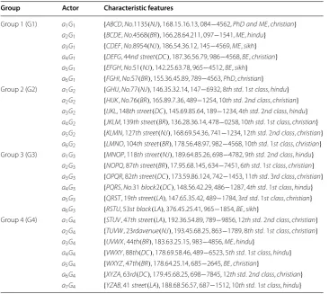
Table 3 Actors and their characteristic features used in the museum social network
Group Actor Characteristic features
Group 1 (G1) a1G1 {ABCD,No.1135(NJ), 168.15.16.13, 084−4562,PhD and ME,christian} a2G1 {BCDE,No.4568(BR), 166.28.64.211, 097−1541,ME,hindu}
a3G1 {CDEF,No.8954(NJ), 186.54.36.12, 145−4569,ME,sikh}
a4G1 {DEFG, 44nd street(DC), 187.36.56.79, 986−4568,BE,christian} a5G1 {EFGH,No.51(NJ), 142.25.63.78, 965−4512,BE,sikh}
a6G1 {FGHI,No.57(BR), 155.36.45.89, 789−4563,PhD,christian} Group 2 (G2) a1G2 {GHIJ,No.77(NJ), 146.35.32.14, 147−6932, 8th std. 1st class,hindu}
a2G2 {HIJK,No.76(BR), 165.89.7.36, 489−1254, 10th std. 2nd class,christian}
a3G2 {IJKL, 148th street(DC), 145.69.85.64, 189−1234, 4th std. 2nd class,hindu}
a4G2 {JKLM, 139th street(BR), 136.28.36.14, 478−0258, 10th std. 1st class,christian} a5G2 {KLMN, 127th street(NJ), 168.69.54.36, 741−1234, 12th std. 2nd class,christian}
a6G2 {LMNO, 104th street(BR), 178.56.48.97, 982−4568, 10th std. 1st class,christian} Group 3 (G3) a1G3 {MNOP, 118th street(NJ), 189.64.85.26, 698−4782, 9th std. 2nd class,hindu}
a2G3 {NOPQ, 87th street(BR), 17.95.68.145, 634−7451, 6th std. 1st class,christian}
a3G3 {OPQR, 82th street(DC), 173.59.86.124, 742−1453, 11th std. 3rd class,christian}
a4G3 {PQRS,No.31block2(DC), 148.56.42.29, 486−1287, 4th std. 1st class,hindu}
a5G3 {QRST, 19th street(LA), 147.65.35.42, 489−1784, 3rd std. 1st class,christian}
a6G3 {RSTU, 53st block(LA), 376.45.25.41, 965−1854,BE,sikh}
Group 4 (G4) a1G4 {STUV, 47th street(LA), 192.36.54.89, 789−9856, 12th std. 2nd class,christian}
a2G4 {TUVW, 23rdavenue(NJ), 193.45.68.25, 863−1789, 8th std. 1st class,christian}
a3G4 {UVWX, 44th(BR), 183.63.25.15, 983−4856,ME,hindu}
a4G4 {VWXY, 88th(DC), 178.69.58.46, 489−6523, 5th std. 1st class,hindu}
a5G4 {WXYZ, 47th(BR), 178.64.25.14, 685−2645,BE,christian}
a6G4 {XYZA, 63rd(DC), 179.45.68.25, 698−7845, 12th std. 2nd class,christian}
a7G4 {YZAB, 41street(LA), 188.68.56.57, 687−1512, 10th std. 1st class,hindu}
Table 4 Actors along with their common characteristic features, weights, and relations used in the ASN
Actors Common characteristic features Weight of actors Relation
among actors
1. PS and JS1 pro1
PS=PhD=23,pro1JS1=ME=18,
pro4PS=pro4JS1=collector=e2,
actPS2 =actJS21=publications=2
WPS=8.0972, WJS1=6.8472 WPS>WJS1 Hierarchical relation
2. PS and JS2 pro1
PS=PhD=23,pro1JS2=ME=18,
pro4PS=pro4JS2=collector=e2,
actPS2 =actJS22=publications=2
WPS=8.0972,WJS2=6.8472 WPS>WJS2
Hierarchical relation
3. JS1 and JS2 pro1
JS1=pro1JS2=ME=18,pro4JS1
=pro4JS2=collector=e2,act2JS1
=actJS22=publications=2
WJS1=6.8472,WJS2=6.8472 WJS1=WJS2 Equivalence relation
4. JS1 and PA1 pro1
JS1=ME=18,pro1PA1
=BE=16,pro3JS1=pro3PA1
=conference=0.8632
WJS1=4.7158,WPA1=4.2158 WJS1>WPA1 Hierarchical relation
5. JS2 and PA2 pro1JS2=ME=18,pro1PA2=BE
=16,pro4JS2=pro4PA2=collector =e2,actJS22=actPA22=publications=2
Also, JS1 and PA1 have common professional information (ProIJS1∩ProIPA1�=φ)
such as ME and BE, and conference.
Since, WJS1>WPA1, the hierarchical relation exists among the actors JS and PA1. Hence,
the hierarchical relation exists among the actors PS, JS1, and PA1 as shown in Fig. 6.
Equivalence relation among actors in the agriculture social network
Consider actors PS, JS1, and JS2, where PS and JS1 have common professional infor-mation (ProIPS∩ProIJS1�=φ and activity ActPS∩ActJS1�=φ) such as PhD and ME,
col-lector, and publications. Similarly PS and JS2 have common professional information (ProIPS∩ProIJS2�=φ and activity ActPS∩ActJS2�=φ) such as PhD and ME, collector,
and publications.
Since, WPS >WJS1, WPS>WJS2, and WJS1=WJS2, the equivalence relation exists among the actors JS1 and JS2 as shown in Fig. 6. Also, WPA1�=WPA2, hence the equivalence relation doesn’t exists among the actors PA1 and PA2.
WJS1=
pro1JS1+pro 3 JS1
4 =
18+0.8632
4 =4.7158
WPA1=
pro1PA1+pro
3
PA1
4 =
16+0.8632
4 =4.2158
WPS=
pro1PS+pro4PS+actPS2
4 =
23+e2+2
4 =8.0972
WJS1=
pro1JS1+pro 4 JS1+act
2 JS1
4 =
18+e2+2
4 =6.8472
WJS2=
pro1JS2+pro 4
JS2+act 2
JS2
4 =
18+e2+2
4 =6.8472
WPA2=
pro1PA2+pro 4
PA2+act 2 PA2
4 =
16+e2+2
4 =6.3472
Relation among actors in the museum social network
We consider the MSN as another example (see Fig. 5), where some of the actors along with their common characteristic features, weights, and relations used in the MSN are shown in Table 5.
Simulation environment
We have considered characteristic features of actors and four groups of actors of agricul-ture and museum social network as shown in Fig. 7 to simulate the GAMPSON. Initially all actors are assigned their respective personally identifiable information, professional information, activity, history, and social status. As actors enter the system randomly, the GAMPSON dynamically monitors different characteristic features depending upon cir-cumstances of actors, and corresponding relations among actors are formed. We also provided access to actors over databases based on the relation among the actors.
Simulation Results
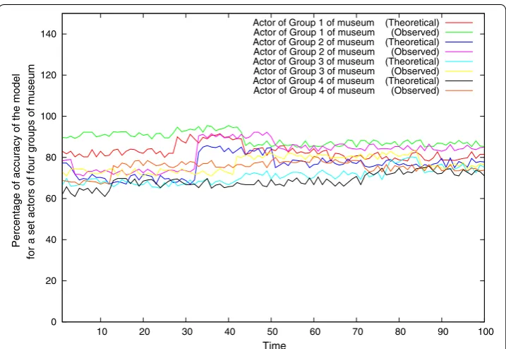
We have created profiles of actors of ASN and MSN based on actors characteristic fea-tures, and calculated weights of actors theoretically. Later, using the GAMPSON, the variation of weights of actors is observed over time through simulations (on Java plat-form). We have varied characteristic features of the actors of ASN and MSN consider-ing Eq. 2 and taken the average of values (we call it theoretical value). Later, we observe characteristic features for one path, and compare with the average value (we call it observed). The results are shown in Figs. 8 and 9, where the graphs are plotted as the percentage of accuracy (obtained from Eq. 3) of the model for a set of actors of a group against time for ASN and MSN, respectively, and show that the theoretical and observed weights of actors matches closely.
Other graphs are plotted in Figs. 10 and 11 for the percentage of accuracy of the model for a set of actors of four groups against time for ASN and MSN, respectively, and show (3) Accuracy= True value of relation−Variation in true value of relation
True value of relation
Table 5 Actors along with their common characteristic features, weights, and relations used in the MSN
Actors Common characteristic
features Weight of actors Relation among actors
1. a1G1 and a2G1 pro1a1G1=PhD=23,
pro1a2G1=ME=18
Wa1G1=5.75,Wa2G1=4.5 Wa1G1>Wa2G1 Hierarchical relation
2. a1G1 and a3G1 pro1
a1G1=PhD=23,
pro1a3G1=ME=18
Wa1G1=5.75,Wa3G1=4.5 Wa1G1>Wa3G1
Hierarchical relation
3. a2G1 and a3G1 pro1a
2G1=pro
1
a3G1=ME=18 Wa2G1=4.5,Wa3G1=4.5 Wa2G1=Wa3G1 Equivalence relation 4. a2G1 and a4G1 pro1a2G1=ME=18,
pro1
a4G1=BE=16
Wa2G1=4.5,Wa4G1=4 Wa2G1>Wa4G1 Hierarchical relation
5. a3G1 and a5G1 pro1a3G1=ME=18,
pro1a5G1=BE=16
Fig. 7 Simulation environment.
0 20 40 60 80 100 120 140
10 20 30 40 50 60 70 80 90 100
Percentage of accuracy of the model for a set of actors of a group of agriculture
Time
Actor 1 of agriculture (Theoretical) Actor 1 of agriculture (Observed) Actor 2 of agriculture (Theoretical) Actor 2 of agriculture (Observed) Actor 3 of agriculture (Theoretical) Actor 3 of agriculture (Observed) Actor 4 of agriculture (Theoretical) Actor 4 of agriculture (Observed)
0 20 40 60 80 100 120 140
10 20 30 40 50 60 70 80 90 100
Percentage of accuracy of the model
for a set of actors of a group of museum
Time
Actor 1 of museum (Theoretical) Actor 1 of museum (Observed) Actor 2 of museum (Theoretical) Actor 2 of museum (Observed) Actor 3 of museum (Theoretical) Actor 3 of museum (Observed) Actor 4 of museum (Theoretical) Actor 4 of museum (Observed)
Fig. 9 Percentage of accuracy of the model for a set of actors of a group of museum vs time. Here, we have considered a set of actors of a group of museum social network and varied their characteristic features over time.
0 20 40 60 80 100 120 140
10 20 30 40 50 60 70 80 90 100
Percentage of accuracy of the model for a set actors of four groups of agriculture
Time
Actor of Group 1 of agriculture (Theoretical) Actor of Group 1 of agriculture (Observed) Actor of Group 2 of agriculture (Theoretical) Actor of Group 2 of agriculture (Observed) Actor of Group 3 of agriculture (Theoretical) Actor of Group 3 of agriculture (Observed) Actor of Group 4 of agriculture (Theoretical) Actor of Group 4 of agriculture (Observed)
initially significant variation in the weights of the actors, but as time increases, the weights of the actors tend to match closely.
In order to determine the variation of relation for a set of actors over neighbourhood of an actor, we first set up relation among actors theoretically. Later using the GAMP-SON, the variation of relation for a set of actors is observed over neighbourhood of an actor through simulations (on Java platform). We have plotted variation of relation for a set of actors against neighbourhood of the actors. Here, we have considered a path from 1st neighbourhood till 6th neighbourhood and plotted the normalised weight with each actor along the path. Neighbourhood of an actor can be easily seen from Fig. 2, where an actor aj is at first neighbourhood of an actor ai, an actor ak is at second
neigh-bourhood, and so on. Graphs are plotted as the variation of relation for a set of actors of a group against neighbourhood of an actor (Figs. 12, 13) for ASN and MSN, respec-tively, and show that the relation for a set of actors of a group is approximately same up to first neighbourhood for without and with actor model. But as more neighbour-hood of an actor is considered, there is significant improvement in the relation for actors with our actor model than without actor model (from first neighbourhood up to fourth neighbourhood).
Other graphs are plotted in Figs. 14 and 15 for the variation of relation for a set of actors of four groups against neighbourhood of an actor for ASN and MSN, respectively, and again show significant improvement in the relation for actors with our actor model than without actor model (from second neighbourhood up to fourth neighbourhood).
In order to determine accuracy of the model for various actors, we have plotted calcu-lated weights of various actors of a group and also of four different groups. Bar graphs in
0 20 40 60 80 100 120 140
10 20 30 40 50 60 70 80 90 100
Percentage of accuracy of the model
for a set actors of four groups of museum
Time
Actor of Group 1 of museum (Theoretical) Actor of Group 1 of museum (Observed) Actor of Group 2 of museum (Theoretical) Actor of Group 2 of museum (Observed) Actor of Group 3 of museum (Theoretical) Actor of Group 3 of museum (Observed) Actor of Group 4 of museum (Theoretical) Actor of Group 4 of museum (Observed)
0 0.2 0.4 0.6 0.8 1
0 1 2 3 4 5 6
Variation of relation for a set of actors of a group of agriculture
Neighbourhood of an actor
Actor 1 of agriculture (Without actor model) Actor 1 of agriculture (With actor model) Actor 2 of agriculture (Without actor model) Actor 2 of agriculture (With actor model) Actor 3 of agriculture (Without actor model) Actor 3 of agriculture (With actor model) Actor 4 of agriculture (Without actor model) Actor 4 of agriculture (With actor model)
Fig. 12 Variation of relation for a set of actors of a group of agriculture vs neighbourhood of an actor. Here, we have considered a set of actors of a group of agriculture social network and observed the relationship values up to six levels.
0 0.2 0.4 0.6 0.8 1 1.2 1.4
0 1 2 3 4 5 6
Variation of relation for a set of actors of a group of museum
Neighbourhood of an actor
Actor 1 of museum (Without actor model) Actor 1 of museum (With actor model) Actor 2 of museum (Without actor model) Actor 2 of museum (With actor model) Actor 3 of museum (Without actor model) Actor 3 of museum (With actor model) Actor 4 of museum (Without actor model) Actor 4 of museum (With actor model)
0 0.2 0.4 0.6 0.8 1
0 1 2 3 4 5 6
Variation of relation for a set of actors of four groups of agriculture
Neighbourhood of an actor
Actor of Group 1 of agriculture (Without actor model) Actor of Group 1 of agriculture (With actor model) Actor of Group 2 of agriculture (Without actor model) Actor of Group 2 of agriculture (With actor model) Actor of Group 3 of agriculture (Without actor model) Actor of Group 3 of agriculture (With actor model) Actor of Group 4 of agriculture (Without actor model) Actor of Group 4 of agriculture (With actor model)
Fig. 14 Variation of relation for a set of actors of four groups of agriculture vs neighbourhood of an actor. Here, we have considered a set of actors of four groups of agriculture social network and observed the rela-tionship values up to six levels.
0 0.2 0.4 0.6 0.8 1 1.2 1.4
0 1 2 3 4 5 6
Variation of relation for a set of actors of four groups of museum
Neighbourhood of an actor
Actor of Group 1 of museum (Without actor model) Actor of Group 1 of museum (With actor model) Actor of Group 2 of museum (Without actor model) Actor of Group 2 of museum (With actor model) Actor of Group 3 of museum (Without actor model) Actor of Group 3 of museum (With actor model) Actor of Group 4 of museum (Without actor model) Actor of Group 4 of museum (With actor model)
Figs. 16 and 17 show the comparison of the normalised percentage of the accuracy of the model for a set of actors of a group and indicates that the normalised accuracy values for actors of ASN and MSN varies between 18 to 86% and 10 to 82%, respectively.
The comparison for the normalised percentage of accuracy of the model for a set of actors of four groups are shown in bar graphs Figs. 18 and 19 for ASN and MSN, respec-tively, and also explains that the maximum accuracy values for group 1, group 2, group 3 and group 4 are 82, 80, 68 and 62%, respectively for ASN and the maximum accuracy values for group 1, group 2, group 3 and group 4 are 83, 80, 66 and 64%, respectively for MSN.
In order to determine accuracy of the model for a set of actors of a group for cross social networks, we have taken actors of ASN and applied to MSN, and vice versa. The graph is plotted in Fig. 20 as percentage of accuracy of the model for a set of actors of a group of agriculture applied to museum against time, and shows large variation in theo-retical and observed values over time. Another graph is plotted in Fig. 21 as percentage of accuracy of the model for a set of actors of a group of museum applied to agriculture against time, and also shows significant variation in theoretical and observed values over time.
The graph is plotted in Fig. 22 as percentage of accuracy of the model for a set actors of four groups of agriculture applied to museum against time, and shows large varia-tion in theoretical and observed values over time. Another graph is plotted in Fig. 23 as percentage of accuracy of the model for a set actors of four groups of museum applied to agriculture against time, and also again shows large variation in theoretical and observed values over time.
0 0.2 0.4 0.6 0.8 1
10 20 30 40 50 60 70 80 90 100
Normalised percentage of accuracy of the model
for a set of actors of agricultur
e
Actor
0 0.2 0.4 0.6 0.8 1
10 20 30 40 50 60 70 80 90 100
Normalised percentage of accuracy of the model
for a set of actors of a group of museum
Actor
Fig. 17 Normalised percentage of accuracy of the model for a set of actors of a group of museum vs actor. Here, we have considered a set of actors of museum social network and observed percentage of accuracy of our model for hundred actors.
Fig. 19 Normalised percentage of accuracy of the model for a set of actors of four groups of museum vs actor. Here, we have considered a set of actors of four groups of museum social network and observed per-centage of accuracy of our model for actors.
0 20 40 60 80 100 120 140
10 20 30 40 50 60 70 80 90 100
Percentage of accuracy of the model
for a set of actors of a group of agriculture applied to museum
Time
Actor 1 of agriculture applied to museum (Theoretical) Actor 1 of agriculture applied to museum (Observed) Actor 2 of agriculture applied to museum (Theoretical) Actor 2 of agriculture applied to museum (Observed) Actor 3 of agriculture applied to museum (Theoretical) Actor 3 of agriculture applied to museum (Observed) Actor 4 of agriculture applied to museum (Theoretical) Actor 4 of agriculture applied to museum (Observed)
0 20 40 60 80 100 120 140
10 20 30 40 50 60 70 80 90 100
Percentage of accuracy of the model
for a set of actors of a group of museum applied to agriculture
Time
Actor 1 of museum applied to agriculture (Theoretical) Actor 1 of museum applied to agriculture (Observed) Actor 2 of museum applied to agriculture (Theoretical) Actor 2 of museum applied to agriculture (Observed) Actor 3 of museum applied to agriculture (Theoretical) Actor 3 of museum applied to agriculture (Observed) Actor 4 of museum applied to agriculture (Theoretical) Actor 4 of museum applied to agriculture (Observed)
Fig. 21 Percentage of accuracy of the model for a set of actors of a group of museum applied to agriculture vs Time. Here, we have varied characteristic features of a set of actors of a group of museum social network and applied them over agriculture social network in order to observe accuracy over time.
0 20 40 60 80 100 120 140
10 20 30 40 50 60 70 80 90 100
Percentage of accuracy of the model
for a set actors of four groups of agriculture applied to museum
Time
Actor of Group 1 of agriculture applied to museum (Theoretical) Actor of Group 1 of agriculture applied to museum (Observed) Actor of Group 2 of agriculture applied to museum (Theoretical) Actor of Group 2 of agriculture applied to museum (Observed) Actor of Group 3 of agriculture applied to museum (Theoretical) Actor of Group 3 of agriculture applied to museum (Observed) Actor of Group 4 of agriculture applied to museum (Theoretical) Actor of Group 4 of agriculture applied to museum (Observed)
In order to observe accuracy of the model for various actors for cross social networks, we have plotted calculated weights of various actors of a group and also of four different groups. Bar graphs in Figs. 24 and 25 show the comparison of the normalised percentage of accuracy of the model for a set of actors of a group, and indicates that the normalised accuracy values for actors of ASN and MSN varies between 18 and 92% and 10 and 85%, respectively.
The comparison for the normalised percentage of accuracy for a set of actors of four groups for cross social networks are shown in bar graphs Figs. 26 and 27, respectively, and also explains that the maximum accuracy values for group 1, group 2, group 3 and group 4 are 78, 72, 52 and 46%, respectively for actors of ASN applied to MSN and the maximum accuracy values for group 1, group 2, group 3 and group 4 are 66, 56, 50 and 38%, respectively for actors of MSN applied to ASN.
Comparison of percentage of accuracy of the GAMPSON, ICT [43], and Stochas-tic model [38] over actors of agriculture social network and museum social network is shown in Figs. 28 and 29, and comparison of cross social networks is shown in Figs. 30 and 31. In all the cases, GAMPSON accuracy is better (see Table 6) than ICT and Sto-chastic model. Average accuracy for the GAMPSON, ICT, and StoSto-chastic model is 71–82%, 56–66%, and 49–64%, respectively.
Comparison of variation of relation for the GAMPSON, ICT, and Stochastic model over actors of agriculture social network and museum social network is shown in Figs. 32 and 33, and comparison of cross social networks is shown in Figs. 34 and 35. In all the cases, GAMPSON is efficient in finding relations better (see Table 7) than ICT and Stochastic model.
0 20 40 60 80 100 120 140
10 20 30 40 50 60 70 80 90 100
Percentage of accuracy of the model
for a set actors of four groups of museum applied to agriculture
Time
Actor of Group 1 of museum applied to agriculture (Theoretical) Actor of Group 1 of museum applied to agriculture (Observed) Actor of Group 2 of museum applied to agriculture (Theoretical) Actor of Group 2 of museum applied to agriculture (Observed) Actor of Group 3 of museum applied to agriculture (Theoretical) Actor of Group 3 of museum applied to agriculture (Observed) Actor of Group 4 of museum applied to agriculture (Theoretical) Actor of Group 4 of museum applied to agriculture (Observed)
0 0.2 0.4 0.6 0.8 1
10 20 30 40 50 60 70 80 90 100
Normalised percentage of accuracy of the model
for a set of actors of a group of agriculture applied to museum
Actor
Fig. 24 Normalised percentage of accuracy of the model for a set of actors of a group of agriculture applied to museum vs actor. Here, we have considered a set of actors of agriculture social network and applied them over museum social network in order to observe percentage of accuracy of our model for hundred actors.
0 0.2 0.4 0.6 0.8 1
10 20 30 40 50 60 70 80 90 100
Normalised percentage of accuracy of the model
for a set of actors of a group of museum applied to agriculture
Actor
Fig. 26 Normalised percentage of accuracy of the model for a set of actors of four groups of agriculture applied to museum vs group. Here, we have considered a set of actors of four groups of agriculture social network and applied them over museum social network in order to observe percentage of accuracy of our model.
40 50 60 70 80 90 100
10 20 30 40 50 60 70 80 90 100
Comparison of Percentage of accuracy of the GAMPSON, ICT,
and Stochastic model over actors of agriculture
Time
GAMPSON ICT Stochastic
Fig. 28 Comparison of percentage of accuracy of the GAMPSON, ICT, and Stochastic model over actors of agriculture vs time. Here, we have considered a set of actors of agriculture social network and varied their characteristic features over time, and compared percentage of accuracy of the GAMPSON, ICT, and Stochastic model.
40 50 60 70 80 90 100
10 20 30 40 50 60 70 80 90 100
Comparison of Percentage of accuracy of the GAMPSON, ICT,
and Stochastic model over actors of museum
Time
GAMPSON ICT Stochastic
40 50 60 70 80 90 100
10 20 30 40 50 60 70 80 90 100
Comparison of Percentage of accuracy of the GAMPSON, ICT, and Stochastic model over actors of agriculture applied to museum
Time
GAMPSON ICT Stochastic
Fig. 30 Comparison of percentage of accuracy of the GAMPSON, ICT, and stochastic model over actors of agriculture applied to museum vs time. Here, we have varied characteristic features of a set of actors of agriculture social network and applied them over museum social network in order to observe accuracy of the GAMPSON, ICT, and stochastic model over time.
40 50 60 70 80 90 100
10 20 30 40 50 60 70 80 90 100
Comparison of Percentage of accuracy of the GAMPSON, ICT, and Stochastic model over actors of agriculture applied to museum
Time
GAMPSON ICT Stochastic
Conclusions
We considered the problem of building an actor model for a professional social network by exploiting the characteristic features. The main theme of the paper was to address a method of designing a GAMPSON, which facilitated creation of actors by utilising char-acteristic features such as personally identifiable information, professional information, activity, history, and social status. Further more, instead of traditional approach that utilises matrix of data, the proposed system first classified actors into different groups. Secondly, it utilised various characteristics of actors, and relations such as hierarchical and equivalence are built among actors. At last, the GAMPSON was designed for the professional social networks such as ASN and MSN, where the acquisition of the charac-teristic features of actors related to the agriculture and museum were carried out. Rela-tion among actors of the ASN and MSN were dynamically formed and updated. Our simulations demonstrated that the graphs obtained were consistent with the generalised Table 6 Comparison of the GAMPSON, ICT and Stochastic model with respect to accuracy
GAMPSON (%) ICT (%) Stochastic
(%)
1. % of accuracy (for ASN) 83–89 6–72 50–68
2. % of accuracy (for MSN) 71–82 58–68 54 –65
3. % of accuracy (for ASN to MSN) 71– 82 51– 64 48 –61
4. % of accuracy (for MSN to ASN) 58–77 52– 62 45 –61
0 0.2 0.4 0.6 0.8 1
0 1 2 3 4 5 6
Comparison of variation of relation for the GAMPSON, ICT,
and Stochastic model over actors of agriculture
Neighbourhood of an actor
GAMPSON ICT Stochastic
0 0.2 0.4 0.6 0.8 1
0 1 2 3 4 5 6
Comparison of variation of relation for the GAMPSON, ICT,
and Stochastic model over actors of museum
Neighbourhood of an actor
GAMPSON ICT Stochastic
Fig. 33 Comparison of variation of relation for the GAMPSON, ICT, and Stochastic model over actors of museum vs neighbourhood of an actor. Here, we have considered a set of actors of museum social network and observed the relationship values up to six levels, and compared variation of relation for the GAMPSON, ICT, and Stochastic model.
0 0.2 0.4 0.6 0.8 1
0 1 2 3 4 5 6
Comparison of variation of relation for the GAMPSON, ICT,
and Stochastic model over actors of agriculture applied to museum
Neighbourhood of an actor
GAMPSON ICT Stochastic
formulation and the applications. The results are encouraging when we compared the proposed model with the ICT and Stochastic model, and showed that our model performed better in terms of finding relations more accurately. We consider that the Table 7 Comparison of the GAMPSON, ICT and stochastic model with respect to relation
Neighbourhood
1 2 3 4 5 6
1. Variation of relation over neighbourhood (for ASN)
GAMPSON 0.58 0.34 0.26 0.18 0.11 0.03
ICT 0.54 0.25 0.16 0.09 0.05 0.02
Stochastic 0.49 0.22 0.11 0.09 0.04 0.01
2. Variation of relation over neighbourhood (for MSN)
GAMPSON 0.56 0.33 0.25 0.16 0.10 0.02
ICT 0.51 0.27 0.22 0.12 0.06 0.01
Stochastic 0.45 0.22 0.19 0.06 0.01 0.001
3. Variation of relation over neighbourhood (ASN to MSN)
GAMPSON 0.53 0.33 0.23 0.15 0.08 0.01
ICT 0.49 0.24 0.11 0.06 0.02 0.01
Stochastic 0.42 0.21 0.07 0.02 0.01 0.001
4. Variation of relation over neighbourhood (MSN to ASN)
GAMPSON 0.52 0.31 0.23 0.14 0.06 0.01
ICT 0.43 0.26 0.14 0.10 0.04 0.01
Stochastic 0.36 0.21 0.11 0.05 0.01 0.001
0 0.2 0.4 0.6 0.8 1
0 1 2 3 4 5 6
Comparison of variation of relation for the GAMPSON, ICT,
and Stochastic model over actors of museum applied to agriculture
Neighbourhood of an actor
GAMPSON ICT Stochastic
proposed actor model can be used as a tool for automatically constructing a professional social network, and can be easily deployed to find relations among actors meticulously.
The use of actor-oriented approach can change the way in which social networks are constructed and relations among the actors are formed. It can provide practical way to precisely generate actors of any professional social network. The only parame-ters required are the basic once that can be easily acquired through profiles, websites, friends, etc. In the future, we would like to extend our model to find the main character-istic features that reflects the model most and can be used in quick construction of any social network.
Abbreviations
GAMPSON: generic actor model for a professional social network; ASN: agriculture social network; MSN: museum social network; CF: characteristic feature; PerIi: personally identifiable information of the actor ai; ProIi: professional information of the actor ai; Acti: activity of the actor ai; Histi: history of the actor ai; SocSi: social status of the actor ai; Wai: weight of the
actor ai; R(ai,aj): relation among the actors ai and aj. Authors’ contributions
PV conceived the study of the actor model, and participated in its design and coordination and helped to draft the manuscript. SSN carried out the actor model studies, participated in the simulation and drafted the manuscript. All authors read and approved the final manuscript.
Acknowledgements
The authors would like to acknowledge the support and helpful comments of the research scholars of Protocol Engi-neering and Technology Unit, which made the overall presentation better.
Compliance with ethical guidelines Competing interests
The authors declare that they have no competing interests.
Received: 9 February 2015 Accepted: 24 July 2015
References
1. Heidemann J, Klier M, Probst F (2012) Online social networks: a survey of a global phenomenon. Comp Netw 56(18):3866. doi:10.1016/S1389128612003088
2. Greetham DV, Hurling R, Osborne G, Linley A (2011) Social networks and positive and negative affect. Procedias Soc Behav Sci 22(0):4. doi:10.1016/S1877042811013747
3. Qiu J, Lin Z, Tang C, Qiao S (2009) Discovering organizational structure in dynamic social network. In: Ninth IEEE international conference on data mining, ICDM ’09, pp 932–937. doi:10.1109/ICDM.2009.86
4. Ninawe SS, Venkataram P (2013) A method of developing a generic social network. Int J Inf Educ Technol 3:488–493. doi:10.7763/IJIET.2013.V3.323
5. Chen Y, Xu X, Wang Z (2012) Family-oriented social network and services. In: International joint conference on service sciences, IJCSS, pp 217–221. doi:10.1109/IJCSS.2012.25
6. Brodka P, Saganowski S, Kazienko P (2009) GED: the method for group evolution discovery in social networks. Soc Net Anal Min 1–14. doi: 10.1007/s13278-012-0058-8
7. Toivonen R, Kovanen L, Kivel M, Onnela JP, Saramki J, Kaski K (2009) A comparative study of social network models: network evolution models and nodal attribute models. Soc Netw 31(4):240. doi:10.1016/S0378873309000331 8. Jiajin Z, Lichang C, Qingsong D, Haidong Z, Yonghua Z (2014) A social networks integrated sensor platform for
preci-sion agriculture. In: 4th IEEE international conference on network infrastructure and digital content, IC-NIDC, pp 131–136. doi:10.1109/ICNIDC.2014.7000280
9. Huatao P (2010) Path selection for social network evolution map formation of start-up enterprises. In: International conference on computer and communication technologies in agriculture engineering, CCTAE, vol 1, pp 47–50. doi:10.1109/CCTAE.2010.5543709
10. Nunez MM, Aguiar WSP (2014) Efficiency analysis of information technology and online social networks manage-ment: an integrated DEA-model assessment. Inform Manag 51(6):712. doi:10.1016/j.im.2014.05.009.http://www. sciencedirect.com/science/article/pii/S0378720614000627
12. Chen N, Zhang X, Wang C (2015) Integrated open geospatial web service enabled cyber-physical information infra-structure for precision agriculture monitoring. Comp Elect Agri 111(0):7. doi:10.1016/j.compag.2014.12.009.http:// www.sciencedirect.com/science/article/pii/S0168169914003196
13. Wang Y, Wang Y, Qi X, Xu L (2009) OPAIMS: open architecture precision agriculture information monitoring system. In: Proceedings of the 2009 international conference on compilers, architecture, and synthesis for embedded systems. ACM, New York, NY, CASES ’09, pp 233–240. 10.1145/1629395.1629428.http://doi.acm. org/10.1145/1629395.1629428
14. Wilson C, Sala A, Puttaswamy KPN, Zhao BY (2012) Beyond social graphs: user interactions in online social networks and their implications. ACM Trans Web 6(4):17. doi:10.1145/2382616.2382620.http://doi.acm. org/10.1145/2382616.2382620
15. Iribarren JL, Moro E (2011) Affinity paths and information diffusion in social networks. Soc Netw 33(2):134. doi:10.1016/S0378873310000596
16. Lee H, Kwon J (2011) Improving context awareness information retrieval with online social networks. In: First ACIS/ JNU international conference on computers, networks, systems and industrial engineering, CNSI, pp 391–395. doi:10.1109/CNSI.2011.54
17. Valente TW, Fujimoto K, Unger JB, Soto DW, Meeker D (2013) Variations in network boundary and type: a study of adolescent peer influences. Soc Netw 35(3):309. doi:10.1016/S0378873313000154
18. Lin CC, Kang JR, Chen JY (2015) An integer programming approach and visual analysis for detecting hierarchical community structures in social networks. Inform Sci 299(0):296. doi:10.1016/j.ins.2014.12.009. http://www.sciencedi-rect.com/science/article/pii/S0020025514011463
19. Ninawe SS, Venkataram P (2013) A method of designing an access mechanism for social networks. In: Nineteenth IEEE national conference on communications, NCC, pp 1–5. doi:10.1109/NCC.2013.6488048
20. Carminati B, Ferrari E, Perego A (2006) Rule-based access control for social networks. In: On the move to meaningful internet systems 2006: OTM 2006 workshops, Lecture Notes. In: Meersman R, Tari Z, Herrero P (eds) Computer Sci-ence, vol 4278. Springer, Heidelberg, pp 1734–1744
21. Carminati B, Ferrari E, Perego A (2009) Rule-based access control for social networks. ACM Trans Inf Syst Secur 13(1):6. doi:10.1145/1609956.1609962
22. Matharu GS, Mishra A, Chhikara P (2014) A framework to leverage cloud for modernization of Indian agricultural produce marketing system. In: Proceedings of the 2014 international conference on information and communica-tion technology for competitive strategies, ICTCS ’14. ACM, New York, NY, pp 7:1–7:7. doi:10.1145/2677855.2677862. http://doi.acm.org/10.1145/2677855.2677862
23. Peng G, Mu J (2011) Network structures and online technology adoption. IEEE Trans Eng Manag 58(2):323. doi:10.1109/TEM.2010.2090045
24. Schoenebeck G (2013) Potential networks, contagious communities, and understanding social network structure. In: Proceedings of the 22nd international conference on world wide web (International World Wide Web Conferences Steering Committee, Republic and Canton of Geneva, Switzerland, 2013), WWW ’13, pp 1123–1132
25. Wasserman S, Faust K (1994) Social network analysis: methods and applications, vol. 8, Cambridge University Press, Cambridge
26. Lesure RG, Wake TA, Borejsza A, Carballo J, Carballo DM, Lpez IR et al (2013) Swidden agriculture, village longev-ity, and social relations in formative central Tlaxcala: towards an understanding of macroregional structure. J Anthropol Archaeol 32(2):224. doi: 10.1016/j.jaa.2013.02.002. http://www.sciencedirect.com/science/article/pii/ S0278416513000159
27. Armbruster W, Ahearn M (2014) Encyclopedia of agriculture and food Systems. In: Alfen NKV (ed), Academic Press, Oxford, pp 201–219. doi:10.1016/B978-0-444-52512-3.00116-9. http://www.sciencedirect.com/science/article/pii/ B9780444525123001169
28. Chang WL, Lin TH (2010) A cluster-based approach for automatic social network construction. In: IEEE second inter-national conference on social computing, SocialCom, pp 601–606. doi:10.1109/SocialCom.2010.94
29. Malik H, Malik AS ( 2011) Towards identifying the challenges associated with emerging large scale social net-works. Procedia Computer Science. In: The 8th international conference on mobile web information systems, MobiWIS 2011, vol 5, p 58. doi:10.1016/S187705091100384X
30. Daraghmi EY, Ming YS (2012) Using graph theory to re-verify the small world theory in an online social network word. In: Proceedings of the 14th international conference on information integration and web-based applications and services, IIWAS ’12. ACM, New York, NY, pp 407–410. doi:10.1145/2428736.2428811
31. West DB (2000) Introduction to graph theory, 2nd edn. Prentice Hall, London
32. Cutillo L, Molva R, Onen M (2011) Analysis of privacy in online social networks from the graph theory perspective. In: global telecommunications conference, GLOBECOM 2011, IEEE, pp 1–5. doi:10.1109/GLOCOM.2011.6133517 33. Sato I, Yoshida M, Nakagawa H (2008) Knowledge discovery of semantic relationships between words using
non-parametric bayesian graph model. In: Proceedings of the 14th ACM SIGKDD international conference on knowledge discovery and data mining, KDD ’08. ACM, New York, NY, pp 587–595. doi:10.1145/1401890.1401962
34. Jalalimanesh A (2012) Knowledge discovery in scientific databases using text mining and social network analysis. In: IEEE conference on control, systems industrial Informatics, ICCSII, pp 46–49. doi:10.1109/CCSII.2012.6470471 35. Vangala RNK, Hiremath BN, Banerjee A (2014) A theoretical framework for knowledge management in Indian
agricultural organizations. In: Proceedings of the 2014 international conference on information and communication technology for competitive strategies, ICTCS ’14. ACM, New York, NY, pp 6:1–6:7. doi:10.1145/2677855.2677861.http: //doi.acm.org/10.1145/2677855.2677861
36. Yongyuth P, Prada R, Nakasone A, Kawtrakul A, Prendinger H (2010) AgriVillage: 3D multi-language internet game for fostering agriculture environmental awareness. In: Proceedings of the international conference on management of emergent digital ecosystems, MEDES ’10. ACM, New York, NY, pp 145–152. doi:10.1145/1936254.1936280.http://doi. acm.org/10.1145/1936254.1936280
38. Snijders TA, van de Bunt GG, Steglich CE (2010) Introduction to stochastic actor-based models for network dynam-ics. Dynamics of Social Networks. Soc Netw 32(1):44. doi:10.1016/S0378873309000069
39. Yoshida T (2010) Toward finding hidden communities based on user profile. In: IEEE international conference on data mining workshops, ICDMW, pp 380–387. doi:10.1109/ICDMW.2010.20
40. Conti M, Passarella A, Pezzoni F (2012) A model to represent human social relationships in social network graphs, in social informatics, Lecture notes. In: Aberer K, Flache A, Jager W, Liu L, Tang J, Guret C (eds) Computer Science, vol 7710. Springer, Heidelberg, pp 174–187
41. Sabouri H, Sirjani M (2010) Actor-based slicing techniques for efficient reduction of Rebeca models. Selected papers of the 5th international workshop on formal aspects of component software. Sci Comput Program 75(10):811. doi:10.1016/S0167642310000304
42. Lipczak M, Sigurbjornsson B, Jaimes A (2012) Understanding and leveraging tag-based relations in on-line social networks. In: Proceedings of the 23rd ACM conference on hypertext and social media, HT’12. ACM, New York, NY, pp 229–238. doi:10.1145/2309996.2310035
43. Wong I, Steinhoff P (2009) Investigate the social actor model of ICT use in organizations. In: 42nd Hawaii interna-tional conference on system sciences, HICSS ’09, pp 1–8. doi:10.1109/HICSS.2009.274
44. Reddy BS, Srinivas T (2009) Energy use in Indian household sector—an actor-oriented approach. Energy and its sustainable development for India energy and its sustainable development for India. Energy 34(8): 992. doi:10.1016/ S0360544209000437
45. Ghose A, Koliadis G (2007) Actor eco-systems: from high-level agent models to executable processes via semantic annotations. In: 31st annual international computer software and applications conference, COMPSAC 2007. vol. 2, pp 177–184. doi:10.1109/COMPSAC.2007.50
46. Ding J, Cruz I, Li C (2011) A formal model for building a social network. In: IEEE international conference on service operations, logistics, and informatics, SOLI, pp 237–242. doi: 10.1109/SOLI.2011.5986562
47. Choi M, Kim H (2013) Social relation extraction from texts using a support-vector-machine-based dependency trigram kernel. Inform Process Manag 49(1):303. doi:10.1016/S0306457312000544
48. George WAM, Norton N, Alwang J (2015) Economics of agricultural development: world food systems and resource use, 3rd edn. Routledge, Abingdon