R E G U L A R A R T I C L E
Open Access
Predicting and explaining behavioral data
with structured feature space decomposition
Peter G. Fennell
1, Zhiya Zuo
1,2and Kristina Lerman
1**Correspondence:[email protected] 1USC Information Sciences Institute,
Marina del Rey, USA Full list of author information is available at the end of the article
Abstract
Modeling human behavioral data is challenging due to its scale, sparseness (few observations per individual), heterogeneity (differently behaving individuals), and class imbalance (few observations of the outcome of interest). An additional challenge is learning an interpretable model that not only accurately predicts outcomes, but also identifies important factors associated with a given behavior. To address these challenges, we describe a statistical approach to modeling behavioral data called the structured sum-of-squares decomposition (S3D). The algorithm, which is inspired by decision trees, selects important features that collectively explain the variation of the outcome, quantifies correlations between the features, and bins the subspace of important features into smaller, more homogeneous blocks that correspond to similarly-behaving subgroups within the population. This partitioned subspace allows us to predict and analyze the behavior of the outcome variable both statistically and visually, giving a medium to examine the effect of various features and to create explainable predictions. We apply S3D to learn models of online activity from large-scale data collected from diverse sites, such as Stack Exchange, Khan Academy, Twitter, Duolingo, and Digg. We show that S3D creates parsimonious models that can predict outcomes in the held-out data at levels comparable to state-of-the-art approaches, but in addition, produces interpretable models that provide insights into behaviors. This is important for informing strategies aimed at changing behavior, designing social systems, but also for explaining predictions, a critical step towards minimizing algorithmic bias.
Keywords: Computational social science; Empirical studies; Online social networks; Human behavior; Feature selection
1 Introduction
Explanation and prediction are complementary goals of computational social science [1]. The former focuses on identifying factors that explain human behavior, for example, by using regression to estimate parameters of theoretically-motivated models from data. In-sights gleaned from such interpretable models have been used to inform the design of social platforms [2] and intervention strategies that steer human behavior in a desired di-rection [3]. In recent years, prediction has become the de-facto standard for evaluating learned models of social data [4]. This trend, partly driven by the dramatic growth of be-havioral data and the success of machine learning algorithms, such as decision trees and
support vector machines, emphasizes ability to accurately predict unseen cases (out-of-sample or held out data) over learning interpretable models [5,6].
Explainability, however, has become an important aspect of computational modeling. Increasingly, applications of machine learning in commercial, educational, and even ju-dicial settings (e.g., [7]) are subject to regulation and to scrutiny for adverse effects such as biases and discrimination. For example, the US Equal Credit Opportunity Act requires creditors to provide an explanation to an applicant when their models recommend reject-ing the applicant for credit, and such explanations require model interpretability. Mean-while, controversy around discrimination in algorithmic decisions (e.g., see [8]) have fur-ther highlighted the need for transparent models whose recommendations can be un-derstood, in contrast to black box algorithms where the step from input data to output decision is opaque. As we come to rely on algorithms to make decisions big and small, the need for algorithmic transparency and the ability to explain machine predictions become ever more acute.
Interpreting algorithms and making sense of behavioral data, however, has proven chal-lenging. Behavioral data is usually massive, containing records of many individuals, each with a large number of potentially highly correlated features. However, the data is also sparse (with only a few observations available per individual) and unbalanced (few ex-amples of the behavior within each class). Yet another challenge is heterogeneity: data is composed of subgroups that vary widely in their behavior. For example, the vast bulk of social media users have very few followers and post a few messages, but a few users have millions of followers or are extremely prolific posters. Ignoring heterogeneity can lead an-alysts to wrong conclusions due to statistical paradoxes [9,10].
Machine learning, data science, and social science communities have proposed a num-ber of approaches to learning explainable models from data. Popular among these are re-gression methods and decision trees, and their ensemble variants, such as random forests and boosting methods. However, while these approaches address one set of challenges, they often trip over the remaining ones. Regression models (e.g., Ridge, Lasso, Elastic Net), while offering interpretability, are limited by their specified functional form and fail to cap-ture relationships in data that do not adhere to this form, and thus can be ineffective at adequately representing the data. Tree-based methods, on the other hand, are very effec-tive at capturing non-linear and unbalanced data, but have limited interpretability. While they offer a measure of feature importance, the relationship between the outcome and features is less transparent, as it requires navigating the depths of many trees, potentially with the same features appearing at different levels.
Motivated by the need for algorithms that perform strongly at both joint goals of pre-diction and explanation, we proposeStructured Sum-of-Squares Decomposition(S3D) al-gorithm, a mathematically principled method for learning interpretable statistical models of behavioral data. The algorithm, which is a variant of decision trees [11], builds a sin-gle tree-like structure that is both highlyinterpretableand can be used for out-of-sample
prediction. In addition, the learned models can be used tovisualizedata.
not selected by the model. Similar to decision trees, the S3D algorithm recursively bins the
m-dimensional space defined by the selected features into smaller, more homogeneous subgroups or bins, where the outcome variable exhibits little variation within each bin but significant variation between bins. However, in contrast to decision trees, it does so in a structured way, by minimizing variation in the outcomeconditionedon the existing partition. The decomposition effectively creates an approximation of the (potentially non-linear) functional relationship betweenYand the features, while the structured nature of the decomposition gives the model interpretability and also helps reduce overfitting. The resulting model is parsimonious. Indeed, S3D is a low complexity model with only two hyperparameters, but despite its low complexity we show that it is a highly performant predictive tool.
To demonstrate the utility of the proposed method, we apply it to model a variety of datasets, from benchmarks to large-scale heterogeneous behavioral data that we collect from social platforms, including Twitter, Digg, Khan Academy, Duolingo, and Stack Ex-change. Across datasets, the performance of S3D is competitive to existing state-of-the-art methods on both classification and regression tasks, while it also offers several advantages. We highlight these advantages by showing how S3D reveals the important factors in ex-plaining and predicting behaviors on the question answering site Stack Exchange and so-cial network Digg. Qualitatively, S3D allows for visualizing the relationship between the outcome and features, and quantifies their importance via prediction task. Surprisingly, despite high heterogeneity of these relationships in many datasets, just a few important features identified by S3D can predict held-out data with remarkable accuracy.
The paper is laid out as follows. In Sect.2we examine related work. In Sect.3we intro-duce the S3D model and describe the algorithm for training the model from data. Section4 is the results section where we apply S3D to various datasets, comparing itsaccuracyto state-of-the-art models while also using itsinterpretabilityto examine and understand data. We conclude in Sect.5. We expect that S3D can be a high utility tool to interpretable modelling in both the scientific and commercial domains, and so have made our code open source to the community at large [12].
2 Related work
An empirical study of socio-behavioral data typically begins with a researcher selecting a small set of explanatory variables—perhaps those identified by Principal Component Analysis (PCA), factor analysis, or a more complex method—and a functional form of the relationship between these and the outcome variable, and performs regression analysis to find the coefficients of the explanatory variables. S3D is a novel approach to predictive analytics that combines the necessities of data modeling in a single method: dimensionality reduction, predictive power and iterpretability.
variation of the outcome variable. Indeed different outcomes variables can result in ferent subsets of features, in contrast to unsupervised methods. Another factor that dif-ferentiates PCA from S3D is that PCA-learned components are in the derived eigenspace of the features, and thus, they are not directly interpretable within domain knowledge. In contrast, S3D selects important features directly in the same space, which aids interpre-tation.
S3D also builds a predictive model of data. Social science, machine learning and data science communities have developed a variety of solutions for this task. However, while these solutions address one set of challenges, they often trip over the remaining ones. Linear models, such as linear and logistic regression, have been the mainstay of the com-putational social sciences community for decades, due to their ability to provide inter-pretable models of data. However, linear models have a number of drawbacks that limit their utility. They are constrained by their functional form and cannot capture non-linear relationships and complex interactions between features. Furthermore, the interpretabil-ity of the coefficients of a linear model can be very limited in data with correlated features. Normally, a researcher examines the effect of a feature on the outcome variable through inspection of the linear coefficient of the feature in the model, but such analysis assumes independence of the features (so that other features can remain constant given a change in the feature). Thus, such analysis with correlated features is not good practice and can lead to misleading conclusions. A standard avenue for improving a linear model is through penalized regression, such as Lasso, Ridge and Elastic Net [13] to reduce the dimension-ality of the feature space and to prevent overfitting [14]. These methods select important features for explaining the data, but are not guaranteed to pick features that are uncorre-lated. Furthermore, such approaches can also set the coefficients of the remaining features to zero, which makes it impossible to learn how those features affect behavior. In contrast, S3D explicitly learns relationships between correlated features from data and can express these relationships through a network, giving insights into the interdependency between selected and remaining features. Unlike linear models, it can also learn non-linear rela-tionships in data.
Machine learning methods are often significantly more accurate than simpler linear models. While deep learning has attracted attention recently due to its performance on highly complex tasks in natural language processing, computer vision and robotics, tree-based algorithms typically perform as well, if not better, on traditional tasks involving tab-ular data. These algorithms are based on decision trees, such as CART [11], BART [15] or MARS [16], which work by partitioning data into non overlapping bins to minimize the variance of response variable, or some other cost function, within these subsets. De-cision trees are typically prone to overfitting (e.g., early stopping and pruning) and so are ensembles to create optimal models. Ensemble approaches include boosting models such XGBoost or LightGBM, and bagging models the most well known of which is random forest models [17]. Random forest models, for example, learn a model as an average of individual decision trees trained on subsets of the data, and averaging in this way reduces overfitting and optimizes performance on held-out test sets.
While a decision hierarchy may be considered interpretable [18], many factors can com-plicate interpretability, such as the depth of the tree and the fact that the same feature can appear at multiple levels. As a result, one does not look too deeply in the tree—generally, at the features at the first level only. In contrast, S3D does not reuse features at different lev-els of the hierarchy, which lends itself naturally to visualization. As we show in this paper, the aerial views of the important feature space serve to provide not just interpretability, but insight into data.
In summary, S3D combines the performance of high accuracy tree-based methods with the interpretability of regression. It carries out dimensionality reduction and feature selec-tion as part of the model fitting stage, and can fit a variety of implicit funcselec-tional relaselec-tion- relation-ships between the variables, not just the linear relationship. S3D’s predictions of binary outcomes are not as sensitive to parameter choices as BART’s [19]. It has much lower complexity than tree-based methods which typically employ tens or hundreds of trees; indeed S3D also has the advantage of having only two parameters to tune, as opposed to twelve for a typical random forest. S3D adds structure to the feature importance offered by random forests, showing which subset of features are sufficient for explaining varia-tion in outcomes. Finally, S3D is fully transparent and allows for visualizing the data and predictions. S3D addresses interpretability by identifying features that are important to explaining the outcome variable, along with the relationship between these features and the outcome. This feature identification can help inform mathematical models of human behavior. Such model-based approaches have been used, for example, to predict popular-ity of online content [20], the productivity of scientists [21], and the size of epidemics [22].
3 Method
We present the Structured Sum-of-Squares Decomposition algorithm (S3D), a variant of the classification and regression trees (CART) [11,15,16], that takes as input a set of features X ={Xj}Mj=1and an outcome variableY and selects a smaller set ofmimportant
features that collectively best explain the outcome. The method bins the values of each im-portant featureXjSto decompose them-dimensional selected feature space into smaller non-overlapping blocks, such thatYexhibits significant variation between blocks but little variation within each block. These blocks allow us to approximate the functional relation-shipY =f(X) as a multidimensional step function over all blocks in them-dimensional selected feature space, thus capturing non-linear relationships between features and the outcome.
Our method chooses features recursively in a greedy manner, so that features chosen at each step explain most of the variation inY conditionedon the features chosen at the pre-vious steps. Features that are correlated will explain much of the same variation inY, and our approach of successively choosing features based on how much remaining variation inY they explain results in a set XS={XS
j}mj=1 of important features that are orthogonal
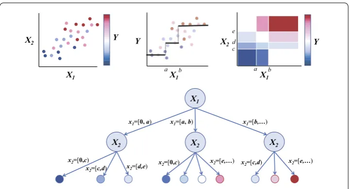
in their relationships withY. By decomposing data recursively, we create a parsimonious model that not only quantifies relationships between the features and the outcome vari-ableY, but also quantifies relationships among the features themselves. Figure1illustrates the algorithm. The left panel shows the data, projected onto the space defined by two fea-turesX1andX2. As the first step, S3D bins the values of each feature and selects one that
explains the largest variation of the outcomeY, hereX1(middle panel). Next, it bins the
Figure 1Illustration of S3D learning a model of data. S3D bins the values of each feature (left panel) to select one that explains the largest variation of the outcomeY(middle panel). Next, it bins each unselected feature to identify one that explains the largest amount of the remaining variation. The aerial view of the partition of the important feature space (right panel) represents a visualization of the data, which is also represented by a tree (bottom panel). S3D continues partition the space using features not previously selected, until there is no appreciable variation left to explain
serves as visualization of the data (right panel). The decomposition of the data according to the selected features can also be represented by a tree (bottom). The algorithm contin-ues in this manner until there is no remaining variation left to explain.
Our model is able to achieve performance comparable to state-of-the-art machine learn-ing algorithms on prediction tasks, while offerlearn-ing advantages over those methods: our al-gorithm uses only two tuning parameters, can represent non-linear relationships between variables, and creates an interpretable model that is amenable to analysis and produces in-sights into behavior that merely predictive models do not give. Below, we described the key steps of the algorithm.
3.1 Structured feature space decomposition
A key concept used to describe variation in observations{yi}Ni=1of a random variableYis
the total sum of squaresSST, which is defined asSST=Ni=1(yi–¯y)2, wherey¯=
N i=1yi/N is the sample mean of the observations. The total sum of squares is intrinsically related to variation inY; indeed the sample varianceσˆ2ofYcan be directly obtained from this quantity asσˆ2=SST/(N– 1).
Given a featureXj, one method of quantifying its importance, i.e., how much variation in Y can be explained byXj is as follows: (1) partitionXjinto a collection PXj of non-overlapping bins (Fig.1), (2) compute the number of data pointsNpand the average value
¯
ypofYin each binp∈PXj, and (3) decompose the total sum of squares ofYas
N
i=1
(yi–¯y)2=
p∈PXj
Np(y¯p–¯y)2+
p∈PXj Np
i=1
(yp,i–¯yp)2, (1)
of squared differences between global (¯y) and local (y¯p) averages that measures how much
Yvaries between different binspofXj. The second sum is the residual sum of squares (or sum of squares within groups), which measures how much variation inYremains within each binp. TheR2 coefficient of determination is then the proportion of the explained
sum of squares to the total sum of squares, given by
R2=
p∈PXjNp(¯yp–y¯)2
SST . (2)
TheR2measure takes values between zero and one, with large values ofR2indicating a
larger proportion of the variation ofYexplained byXj. This method of approximating the functional relationship betweenY andXjas a step function with bins, or groupsPXj and corresponding valuesy¯p, allows us to quantify the variation inY explained byXjthrough theR2of the corresponding step function as given by Eq. (2).
3.1.1 Binning values of a feature
We now introduce a method to systematicallylearnthe binningPXjof the featureXjwhich will be central to our algorithm. Given the data, we can split the domain of the featureXj at the valuesinto two bins:Xj≤sandXj>s. From Eq. (2), we see that the proportion of variation inYexplained by such a split is
R2(s;Xj) =
NXj≤s(y¯Xj≤s–y¯) 2+N
Xj>s(y¯Xj>s–y¯) 2
SST , (3)
where NXj≤s and y¯Xj≤s are the number of data points and average value of Y in the binXj≤s, and vice versa forNXj>sandy¯Xj>s.R2(s;Xj) can be computed for each possi-ble value ofs in the domain ofXj, and we can choose the optimal split s1 as the split
s that maximizes R2(s;X
j) of Eq. (3). Choosing s1, and binning the domain of Xj into
PXj ={[min(Xj),s1], (s1,max(Xj)]}, we can again find the next best splits2 to optimize the improvement inR2. In general, having chosennsplits{s
u}nu=1 with a resulting partition
PXj ofn+ 1 bins, the next best splitsn+1can be chosen as the splitsthat maximizes the improvement inR2as given by
R2(s|PXj;Xj) = 1
SST
Np(s)|Xj≤s(¯yp(s)|Xj≤s) 2
+Np(s)|Xj>s(y¯p(s)|Xj>s) 2–N
p(s)(y¯p(s))2
, (4)
wherep(s) in Eq. (4) is the bin inPXjthat contains the pointsandp(s)|Xj≤s(resp.p(s)|Xj>
s) is the restriction of that bin to pointsXj≤s(resp.Xj>s). In this manner, we recursively split the domain ofXjto create a partition of the feature.
However, splitting in this manner can continue indefinitely, resulting in a model that is too fine-grained and thus overfits the data. To prevent overfitting, we need a stopping criterion. To this end we introduce a loss functionL(PXj) that penalizes the size|PXj|of the partition, i.e., the number of bins:
L(PXj) = 1 –R 2(P
The parameterλcontrols how fine-grained the bins are: smaller values ofλallow for more finer bins, and vice versa. The loss function of Eq. (5) reaches a minimum when the change inR2(P
Xj) from adding an extra split toPXj is less thanλ—at this point we stop splitting and return the binningPXj.
Having formed the binningPXjofXjwith splits{su}
n
u=1, the total scoreR2(Xj) can be cal-culated from Eq. (2), or by summingR2(s1;Xj) from Eq. (3) along with theR2 terms in Eq. (4) for each of the splits{su}nu=2. Completing this procedure for all features gives a
mea-sure offeature importance, i.e., how much variation inYeach feature alone explains, and ranking these features allows us to choose the most important featureXC1 that explains
the largest amount of the variation inY.
3.1.2 Selecting additional features
After choosing the most important feature, we search the rest of the features for one that explains most of the remaining variance inY, then the third feature, and so on. Here, we describe the procedure for finding the next best feature having already chosenlfeatures XS={XS
1, . . . ,XlS}with a corresponding binningPS=PS1× · · · ×PSl of the chosen feature space, where×here is the cartesian product. In this case, a totalR2(PS) =
p∈PSNp(¯yp–
¯
y)2/SSTof the variation inYhas been explained, and we now look for the feature that best
explains the remaining variation 1 –R2(PS).
Given a remaining featureXj, we bin the domain ofXjsimilarly to how we binned it when choosing the first feature. The first splits1 ofXjis chosen as the valuesthat maximizes the improvement inR2, given by
R2s|PS;Xj
= 1
SST
p∈PS
Np|Xj≤s(y¯p|Xj≤s) 2
+Np|Xj>s(y¯Xj>s) 2–N
p(y¯p)2
, (6)
wherep|Xj≤s(resp.p|Xj>s) is the set of data points inp∈PSfor whichXj≤s(resp.
Xj>s). In general, givennsplits and a corresponding partitionPXj ofXj, then+ 1’st split is chosen as the valuesthat maximizes
R2s|PXj,P
S;X j
= 1
SST
p∈PS×P Xj|s∈p
Np|Xj≤s(y¯p|Xj≤s) 2
+Np|Xj>s(y¯Xj>s) 2–N
p(y¯p)2
, (7)
with the sum in Eq. (7) taken over all elementspofPS×P
Xj that contain the points. The loss function in the general setting is
LPXj|P
S=1 –R
2(PS×P Xj)
1 –R2(PS) +λ|PXj|, (8)
where the denominator of the fractional first term in Eq. (8) normalizes this term to be between zero and one, is the case in Eq. (5). This normalization is necessary because as we progress through the algorithm, subsequent features may explain less of the variance ofY(as features are chosen hierarchically), and so changes in 1 –R2(PS×PXj) by splitting
normalization ensures that this is not the case and that the feature is binned consistently at each stage of the algorithm. Again, the partitionPXjofXjis chosen that minimizes the loss function of Eq. (8), and theR2improvement is calculated for this feature as
R2PXj|P
S=R2PS×P Xj
–R2PS. (9)
This procedure is repeated for all remaining featuresXjto select the featureXl+1with the
maximalR2improvement.
This process of binning features, calculating their importance by the improvementR2
and choosing the one with the largest improvement continues until no further variation inYcan be explained or until an alternative stopping condition (such as a pre-specified maximum number of steps) is met. Our algorithm learns a hierarchy of important features that explain the variation inY and a binning or partitionPS with corresponding values
{¯yp}p∈PSapproximating the functional relationship between the outcome and the features. Note that, when binning a feature, once the vectors{{Np|Xj≤s}p∈PS}sand{{¯yp|Xj≤s}p∈PS}s have been constructed (an operation that takesO(N) time), the binning is independent of N, and instead depends on the number of unique values of the feature (as required to calculate the optimal splitssat each step). The fact that S3D scales linearly with the number of data pointsN allows us to apply the algorithm to large datasets, such as the Twitter and Digg (see Sect.4).
3.1.3 Hyperparameters
The S3D model has two hyperparameters: (1)λthat controls granularity of feature bin-ning; (2)kthat specifies the maximum number of features to use for prediction. The hy-perparameterkis analogous to the maximum tree depth in decision tree methods. Both hyperparameters are important to prevent overfitting — left unrestricted, the algorithm can learn too fine-grained a model that fails to generalize to unseen data. We note that it is possible to stop early in the training phase by restricting the maximum number of features to select. In other words, the algorithm can stop when the number of selected features reaches a predefined value. Nonetheless, it is recommendednotto lay any limit during the training phase but rather tunekin the validation step.
To tune the hyperparameters, we train S3D for various values ofλ, in each case letting the algorithm continue until there is no further improvement inR2. This results in a model
withmλselected features and partitionPSλ={P1Sλ, . . . ,PmSλλ}. Then, fork∈[1,mλ], we
eval-uate the predictive performance of the model using only the topkselected features and the sub-partition{PSλ
1 , . . . ,P
Sλ
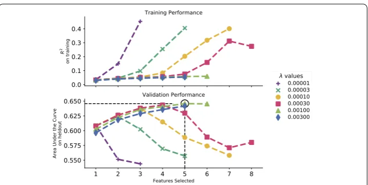
k }(Fig.2). Performance is measured on held-out tuning data using a specified metric. The optimal hyperparameters (λ,k) are those that achieve the best performance on held-out data.
3.2 Applications of the learned model
Given a dataset, S3D learns an ordered set of important, orthogonal features XS, a par-titioningPSof the selected feature space with correspondingy¯
pandNp values for each
bin or blockp∈PS, andR2 for each remaining variable at each step of the algorithm.
Figure 2Hyperparameter tuning onStack Exchangedata. Top:R2in the training set as a function ofλandk;
Bottom: AUC on the held-out data. Note that for illustration, we show the trajectory for only one of five splits. Different “best” hyperparameters may exist for different splits
3.2.1 Feature selection and correlations
The ordered set XSof important, orthogonal features allows us to quantify feature im-portance in heterogeneous behavioral data. The top-ranked features explain the largest amount of variation in the outcome variable, while each successive feature explains most of the remaining variation that is not explained by the features that were already selected. Aside from the selected features XS, S3D provides insights into features that arenot selected by the algorithm, quantifying variation that they explain in the outcome variable that is made redundant through the selected variables. This is calculated in the following manner. At a given steplof the algorithm, featureXSl is selected as the best feature with an
R2improvement ofR2(P
XS l|P
S(l–1)) (Eq. (9)), wherePS(l–1)is the partition prior to stepl.
Meanwhile, a different remaining featureXjhas anR2improvement ofR2(PXj|PS(l–1)). At the next stage of the algorithm, givenXS
l has been selected,Xjwill have anR2improvement ofR2(P
Xj|P
S(l–1)×P
XSl), and thus the variation inXjthat is made redundant through the selection ofXlSis the difference between these twoR2:
aX
j,XlS=R 2P
Xj|P
S(l–1)–R2P
Xj|P
S(l–1)×P
XlS
. (10)
The coefficientsaXj,XS
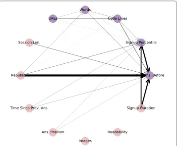
l facilitate our analysis of (a) relationships between the features and (b) the effect of unselected features on the outcome variable (through selected features to which they are correlated). We implement the coefficients as weights in a feature network that is weighted and directed (Fig.8). This network gives a tool for analysis—unselected features that otherwise can explain much of the variation in the outcome will have heavy links, and the selected features XS
l to which these links point reveal correlations and through which selected features the unselected feature is made redundant.
3.2.2 Prediction
continuous-valued outcome variables, this predicted expected valueμˆ will be the pre-diction of the outcome ofY, i.e.,yˆ|x=y¯p(x). For discrete-valued outcomes, the expected
value has to be thresholded to predict an outcome class. For binary outcomesY∈ {0, 1}, ˆ
μ|x=¯yp(x) is the maximum likelihood estimate of the probability of the outcomeY= 1
in the blockp(x), and thus our model specifies that the outcomeY= 1|xwill occur with probabilityy¯p(x). By choosing an appropriatediscrimination thresholdθ, our model then
makes the predictionyˆas
ˆ
y|x=
⎧ ⎨ ⎩
1, y¯p(x)≥θ,
0, y¯p(x)<θ.
(11)
Unbalanced data Two of the datasets that we study, Digg and Twitter, are highly
unbalanced—their outcome variables (whether the useradoptsa meme) are binary, and the proportions of positive outcomes in the data are 0.0025 and 0.0007 respectively. Using the standard discrimination thresholdθ= 0.5 results in predicting an insufficient number of ones. To address this issue, we choose the discrimination threshold based on the train-ing data, picktrain-ing the largest valueθsuch that the number of predicted positive examples in the training data is greater than or equal to the actual number of positive examples in the training set. This threshold is then used for prediction on the held-out tuning data, as well as on the test data. Note that, for these two datasets, we also alter the discrimination threshold for the regression and random forest models in the same manner.
3.2.3 Analysis and model interpretation
One of the more interesting contributions of S3D is its potential for model exploration. By selecting features sequentially, we create a model where typically lower amounts of vari-ation are explained at successive levels, and so a visual analysis of the first few important dimensions of the model allows us to understand the effects of the important features on data and predictions. The expectationsy¯pfor each blockp∈PSfacilitate this exploration, approximating the relationshipY=f(X) between outcome and features. Furthermore, for binary data, the predicted outcomes obtained by thresholding the expectations show how predictions change as a function of the features, which allows for explaining predictions and visually exploring the data.
3.3 Comparison to state-of-the-art
We compare S3D to linear and logistic regression (withLassoandElastic Net[13] regular-ization), random forests (RF) [17], and support vector machines with linear kernel (Linear SVM) [23], using 5-fold cross validation (CV; Section S1.2). The Scikit Learn [24] imple-mentation of the random forest model used in our experiments is based on the CART algorithm. We also compare S3D’s performance to models with similar complexity. First, we use random forest to rank all the features and retrain the model on the top-k(and top-2k) ranked features, wherekis the number of important features selected by S3D. The resulting models are calledRF(k) andRF(2k) respectively. Second, we investigate the ef-ficacy of using S3D forsupervised feature selection. Specifically, we train random forests using only thekimportant features chosen by S3D, which we refer to asRF-S3Dmodel.
Figure 3Classification performance on 5-fold cross validation in nine datasets. Error bars here indicate one standard deviation. A higher bar (greater value) means better performance
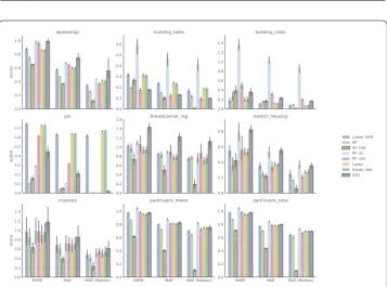
Figure 4Regression performance on 5-fold cross validation in nine datasets. Error bars here indicate one standard deviation. A higher bar (greater value) meansworseperformance
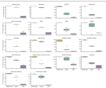
Figure 5Number of features selected by elastic net and lasso regression, as well as S3D, across outer CV for all datasets. The five points in each box correspond to the number of features selected in eachouterfold
We partition data into five equal size folds,aeach of which is rotated as a hold-out set
for testing. For classification (except random forests), we standardize feature values by centering and scaling variance to one. For regression, both features and target values are standardized. Standardization of test set is based on training data. In each run, we train and tune the models on four folds, where three are used for training and one for valida-tion. Finally we evaluate the performance of the tuned models on the remaining test fold. The final evaluation is therefore the average performance across each of the five folds. In other words, we tune the hyperparameters with 4-fold CV (hereafterinner CV) and evaluate the performance of the optimal models with 5-fold CV (hereafterouter CV). For classification tasks, we evaluate performance using (1) accuracy (the percentage of cor-rectly classified data points), (2)F1 score (the harmonic mean of precision, the percent-age of predicted ones that are correctly classified, and recall, the percentpercent-age of actual ones that are correctly classified), and (3) area under the curve (AUC). For regression tasks, we employ (1) root mean squared error (RMSE), (2) mean absolute error (MAE-Mean), (3) median absolute error (MAE-Median). Note that for classification tasks, higher values of the metrics imply better performance. For regression tasks, lower values of the metrics imply better performance. During the inner CV phase (i.e., hyperparameter tuning), we optimize classification performance on AUC scores and regression on RMSE scores.
for each decision tree, and (4) criterion of the quality of a split (choices are Gini impurity or information gain for classification; MAE or MSE for regression). For linear SVM, we tune the penalty parameter for regularization.
4 Results
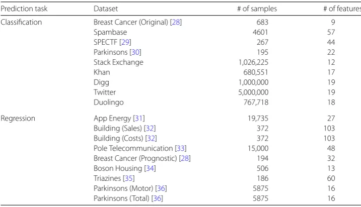
We apply S3Dbto benchmark datasets from the UCI Machine Learning Repository [27]
and from Luís Torgo’s personal website.cIn addition, we include five large-scale behavioral datasets, as described in the following paragraphs. Table1lists all18datasets used in both classification and regression tasks, along with their statistics. See Additional file1Section S1.1 for more detailed description of the benchmark data and data preprocessing.
Behavioral data came from various social platforms:
• Stack Exchange. The Q&A platform Stack Exchange enables users to ask and answer questions. Askers can alsoacceptone of the answers as the best answer. This enables us to measure answerer performance by whether their answer was accepted as the best answer or not. The data we analyze includes a random sample of all answers posted on Stack Exchange from 08/2009 until 09/2014 that preserves the class distribution. Each record corresponds to an answer and contains a binary outcome variableY∈ {0, 1}(one indicates the answer was accepted, and zero otherwise), along with 14 features. These features include answer-based features, such as the length of the answer, measured in the number ofwords,lines of codeandhyperlinksto Web content the answer contains, thenumber of other answersthe question already has, the answer’sreadabilityscore, a numeric index giving the level of education needed to easily comprehend the answer. Other features include the answerer’sreputation, how long the answerer has been registered (signup durationin months) and a percentile rank (signup percentile), the number of answers they have previously written, time since the previous answer, the number of answers written by the answerer in his or her current session, andanswer’s positionwithin the session, i.e., whether it was the first, second, third, etc. answer the user wrote during the same session.
Table 1 Datasets Used for Performance Comparison
Prediction task Dataset # of samples # of features
Classification Breast Cancer (Original) [28] 683 9
Spambase 4601 57
SPECTF [29] 267 44
Parkinsons [30] 195 22
Stack Exchange 1,026,225 12
Khan 680,551 17
Digg 1,000,000 19
Twitter 5,000,000 19
Duolingo 767,718 18
Regression App Energy [31] 19,735 27
Building (Sales) [32] 372 103
Building (Costs) [32] 372 103
Pole Telecommunication [33] 15,000 48 Breast Cancer (Prognostic) [28] 194 32
Boson Housing [34] 506 13
Triazines [35] 186 60
Parkinsons (Motor) [36] 5875 16
• Khan Academy. The online educational platform Khan Academy enables users learn a subject then practice what they learned through a sequence of questions on the subject. We study performance during the practice stage by looking at whether users answered the questions correctly on their first attempt (Y= 1) or not (Y= 0). We study an anonymized sample of questions answered by adult Khan Academy users over a period from 07/2012 to 02/2014. For each question a user answers we have 19 features: as with Stack Exchange, these include answer-based, user-based, and other temporal features. The features include the amount of time it takes the user to answer the question, (solve_time), the number of attempts the user made to answer the question, time since the user’s previous answer (time_since_prev_ans), the number of questions the user answered during the current session, (session_length), and the answer’sposition within the session. Additional features include temporal attributes such as thehourof the day,dayof the week,month, etc. that the question was answered; user-based features, such as the month usersigned upfor Khan Academy, the number offirst_fivequestions user answered correctly without hints, time between user’s first and last answer, (signup_duration), the numbers ofall questions user ever attempted to answer, and the number ofall attemptsmade on all questions, and other features, such as how long this user has currently been studying.
• Duolingo. The online language learning platform Duolingo is accessed through an app on a mobile device. Users are encouraged to use the app in short bursts during breaks and commutes. The datadwas made available as part of a previous study [2]. The data contains a 2-week sample (02/28/2013 through 03/12/2013) of ongoing activity of users learning a language. All users in this data started lessons before the beginning of the data collection period. We focus on 45K users who completed at least five lessons. The median number of lessons was 7, although some had as many as 639 lessons. Performance on a lesson is defined asY= 1if the user gotallthe words in the lesson correct; otherwise, it isY= 0. Features describing the user include how many lessons and sessions the user completed, how many perfect lessons the user had, the month and day of the lesson, etc.
week. Through this data, we can study the factors that are important in explaining the spread of information in this social system.
• Twitter.On the online social network Twitter, users can post information, which is then broadcast to their followers, i.e., the other Twitter users that follow that user. This dataset tracks the spread of 65,000 unique URLs through the Twitter social network during one month in 2010. Similarly toDigg, we can study social influence and information diffusion by examining whether (Y= 1) or not (Y= 0) a user posts a URL after being exposed to it when one of his or her friends posts. The features associated with each exposure event are the same as those forDigg.
We compare the average predictive performance across 5 holdout sets of S3D to Lasso regression, elastic net regression, random forests, and linear SVM. We show that S3D can achieve competitive performance with the benchmark algorithms with a smaller set of features. Finally, we explore our tuned S3D models and demonstrate their utility to understanding human behaviors in Sect.g. Relevant datasets and codesecan be used to
replicate the following results.
4.1 Tuning hyperparameters
An essential part of training a statistical model is hyperparameter tuning—in the case of S3D, selecting the parametersλandk. This procedure is illustrated for Stack Exchange data in Fig.2, where we show the totalR2at each step of the algorithm for various values
ofλ, as well as the AUCs at these steps computed on the held-out tuning data. Overly small values ofλperform quite poorly on the held-out data, as they produce very fine-grained bins that overfit the data. Larger values ofλavoid being too fine-grained—the
R2 on the training set increases initially but diverges again as extra features selected in
additional steps overfit the data (as shown through the decreasing performance on the held-out data; Fig.2bottom). Parameterk(x-axis in Fig.2) controls the number of steps of S3D, thus picking the optimal model between underfitting and overfitting. Supplementary
files3d_hyperparameter_df.csvf reports the best hyperparamters for all datasets, across
the 4-fold inner CV processes.
4.2 Prediction performance
Figures3and4report performance on the outer CV for all datasets S3D, random forests, linear SVM, and logistic regressions (both Lasso and elastic net). Overall S3D achieves predictive performance comparable to other state-of-the-art machine learning methods. In most cases, S3D’s performance is similar to that of logistic regression and linear SVM. Its performance relative to random forest is especially remarkable considering the difference in complexity of the models. S3D uses a subset of features and a simplem -dimensional hypercube to make predictions, in stark contrast to random forests, which use all features and learn many decision trees. In contrast, S3D selects a small set of fea-tures, producing more parsimonious models as compared to Lasso and elastic net regres-sion (Fig.5).
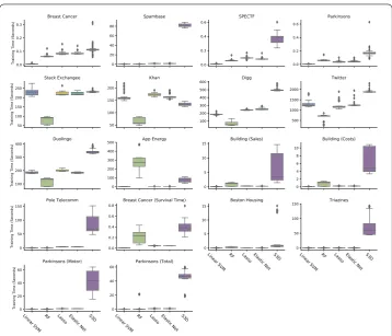
Figure 6Boxplots of training time (seconds) of all five algorithms
Finally, we show that the runtime of S3D is competitive to the other four algorithms (Fig.6). For each dataset, all models were trained using the best parameters found in in-ner CV and full training sets over each split (recall that there are five splits) repeated ten times. In other words, there is no cross validation in the evaluation of runtime, but only in training with the optimal parameters selected in the previous performance evaluation steps. Therefore, each box in Fig.6shows the distribution of training time over 50 runs. Note that the Python package Scikit Learn [24] is used to implement logistic regression, random forest, and linear SVM, therefore producing superb runtime performance, as it is highly optimized. We believe that the implementation of S3D can be further improved. For instance, the timing of S3D includes reading the input file, whereas the other four meth-ods do not require this. Furthermore, Fig.6only reflects training time with one set of hyperparameters for each model. While random forests manifest outstanding efficiency, it is worth noting that the large amount of hyperparameters (in this study, we searched for four; there are at least four more) will inevitably lead to undesirably long hours of grid search. On the other hand, S3D only needs two (λandk), which substantially reduce user effort in hyperparameter tuning.
4.3 Analyzing human behavior with S3D
forDigg. In order to provide the most comprehensive explanation of the data, we applied S3D toall available datausing hyperparameters that were seen most often during cross validation.
4.3.1 Feature selection and correlations
For the large scale behavioral data, S3D selects a subset of features that collectively explain the largest amount of the variation in the outcome variable. It also quantifies correlations between selected features to unselected ones. In the following, we describe selected fea-tures and examine the effects of the unselected ones.
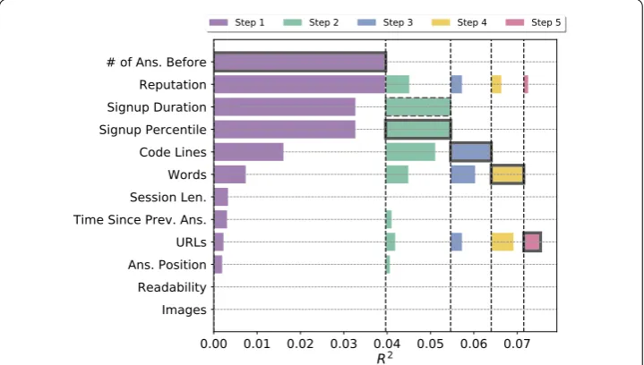
We give a detailed description of the features selected at each step (Fig.7) and the result-ing feature network (Fig.8). Figure7visually ranks the features by showing the amount of variation explained by each feature at every step of the algorithm. The features selected at each step are outlined in black. The first and most important feature selected isthe
num-ber of answers provided before this question. This feature, for one thing, indicates how
active a user is in the community. For another, it implicitly reflects a user’s capability. In-terestingly, there is obvious dependencies between the number of previous answers and
(1)reputation, (2)signup duration/percentile, and (3)code lines. Given the amount of
pre-vious answers in the model, the contribution of these features decreases dramatically. The second feature S3D selects issignup percentile, which measures answerers’ “age” on Stack Exchange as a percentile rank. Intuitively, the longer a user stays in the system, the more likely they can accumulate their reputation and capability to produce a “good” answer. It is noteworthy thatsignup durationandpercentileshare the exact amount of explained vari-ation, which echoes the fact that the Spearman correlation between them is 1. Following user tenure, the number oflines of codesis selected as the third most important feature, followed by thenumber of wordsandURLs, which all, to some extent, manifest how infor-mative an answer is. Note that the variation explained by the featuresnumber of wordsand
Figure 8The feature network for Stack Exchange, showing the variation in the outcome from the features that have not been selected (pink) through the selected features (purple). Edge width is proportional to weights described in Sect.3.2.1—the thicker a link between two features is, the more correlated they are
URLsexceeds the variation explained by these features in the first step, leading to an inter-esting implication that there may exist aninteractioneffect. In particular, given answers with the samenumber of code linesand by answerers who signed up in similar time period and shared similar activeness, thenumber of wordsandURLswill contribute more to the final acceptance probability. The ability to identify moderation effects among variables, in fact, is a fascinating characteristic of S3D when analyzing heterogeneous behavioral data. WithR2= 0.075, the five selected features collectively explain the largest amount of vari-ation in whether an answer is accepted by the asker as the best answer to his or her ques-tion. The unselected features have been made redundant by the selected features. Such redundancies can be represented as a directed and weighted network through the coef-ficients of Equation (10), as shown in Fig.8. Specifically, links between selected features (purple) the unselected (pink) features show the variation in the outcome explained by the pink node can be explained by the purple node. The network visualizes the correlations and the significance of unselected features. While some of the correlations are obvious, such as those between thenumber of answers, user reputation, and tenure length (i.e.,
signup duration/percentile), others are less evident. For example, there are links from
rep-utationto the number ofwords, andcode lines, implying that reputable users may provide
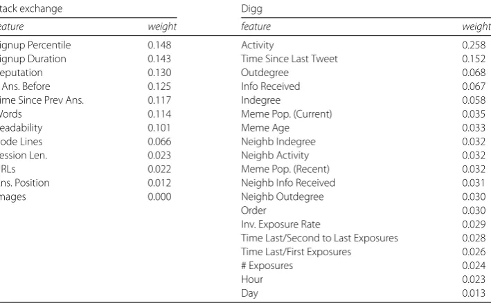
Table 2 Features found to be important by random forest in Stack Exchange and Digg, along with their relative weights
Stack exchange Digg
feature weight feature weight
Signup Percentile 0.148 Activity 0.258
Signup Duration 0.143 Time Since Last Tweet 0.152
Reputation 0.130 Outdegree 0.068
# Ans. Before 0.125 Info Received 0.067
Time Since Prev Ans. 0.117 Indegree 0.058
Words 0.114 Meme Pop. (Current) 0.035
Readability 0.101 Meme Age 0.033
Code Lines 0.066 Neighb Indegree 0.032
Session Len. 0.023 Neighb Activity 0.032
URLs 0.022 Meme Pop. (Recent) 0.032
Ans. Position 0.012 Neighb Info Received 0.031
Images 0.000 Neighb Outdegree 0.030
Order 0.030
Inv. Exposure Rate 0.029
Time Last/Second to Last Exposures 0.028 Time Last/First Exposures 0.026
# Exposures 0.024
Hour 0.023
Day 0.013
early answerers to many questions. The feature network, in this manner, not only lets us analyze which unselected features are explanatory of an outcome variable, but to which selected features they are correlated and are made redundant, providing a tool to suggest further exploration of correlations within the data.
For comparison, features found to be important by the random forest algorithm are shown in Table2, along with their weights. While the top two features selected by S3D for Stack Exchange are also highly ranked by random forest, the latter considers other fea-tures to be more important than the number ofwords,code linesandURLs, which S3D selected as important features. Random forest ranks highly features likeSignup Duration
andReputation, which are highly correlated with existing featuresSignup Percentileand
# Ans. Written by User Before. These correlated features are not useful for prediction, and
may actually hurt performance. This is the reason why some feature selection algorithms, such as minimum redundancy method [37], filter out redundant, highly correlated fea-tures.
In the Khan Academy dataset, S3D selects as important features: (1) thetimeit takes the user to solve the problem; (2) the number of problemsthat the user has solved on the first attempt without hints; (3) time since previous problem; (4) the number offirst
five problemssolved correctly on the first attempt; (5)index of the sessionamong all of
that user’s sessions; (6)index of the problemwithin its session. It is noteworthy that the second and fourth features here are analogous tosignup durationandreputationon Stack Exchange, as the number of problems that a user solves correctly on their first attempt is a combination of both skill and tenure.
In the case of Digg social network, to explain whether a user will “digg” (or “like”) a story recommended by friends, S3D selects as important features: (1) useractivity(how many stories this user recommended); (2) the amount ofinformation receivedby this user from the people she follows; (3) current popularity of this story, and (4) user in-degree. The first two features describe how a user processes and receives information, while the third one reflects how “viral” a story is, and fourth features is how many people the user follows. The features selected by S3D are also ranked highly by random forest (Table2); although, features highly correlated with these, such astime since last tweet, which is correlated with
useractivity, andindegree, which is correlated with the amount ofinformation received,
are ranked equally high. Since their effect is already captured by the selected features, they are not needed in the model.
For Twitter, S3D selects (1) the amount ofinformation receivedby this user; (2)in-degree
(i.e., the number of followers and thus popularity) of friends; (3) the number oftimesthis user has been exposed to this meme; (4) useractivity; (5) the age of this tweet; (6) user’s
out-degree(followees). S3D identifies the information received by the user as an important
feature for both Digg and Twitter, which highlights important role that cognitive load plays in information spread online [38]. On the other hand, the differences such as the lesser importance of user activity and greater importance of a user’s friends in Twitter suggests interesting disparities in the manner of information diffusion on these two platforms.
4.3.2 Model analysis
S3D is a promising tool for data exploration. By iteratively selecting features and measur-ing the amount of outcome variation they explain (Fig.7), we can visualize the important dimensions of the model to fully understand both effects of important features and the corresponding predictions. See Additional file1for a detailed step-by-step illustration.
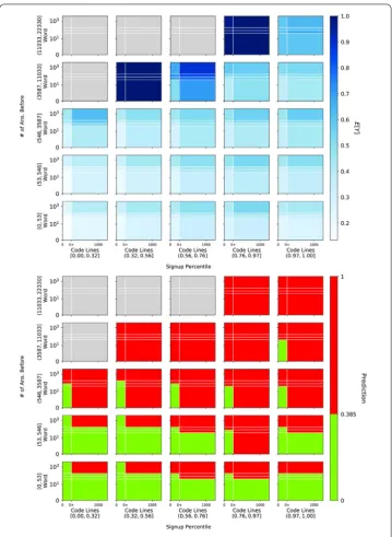
For Stack Exchange, S3D selects five important features. We visualize the model with the first four features in Fig.9, that unfolds them= 4 hypercube learned by the model. It shows how the expectation (top plot) and the corresponding prediction (bottom plot) that the answer will be accepted as best answer, vary as a function of the four selected features. The prediction threshold selection is described in Sect.3.2.2. Each row of plots in Fig.9corresponds to a single bin of the first selected featurenumber of answers before, while each column corresponds to bins of the second featuresignup percentile rank. Indi-vidual plots vary according to the third and fourth featurescode linesandwords. It is quite evident that variation in the outcome (i.e., Fig.9top plot) is greater between plots than within plots, a result of the fact that features are pickedsuccessivelyto explain such vari-ation. These plots show the collective effects of these four features: acceptanceincreases
with the user’s experience (number of answers beforefeature) and tenure (signup percentile rank). Furthermore, longer answers with morewordsandlines of codeare more likely to be accepted as best answers. Another interesting pattern emerges when the number of answers provided before is above 3587: the acceptance rate rises whensignup percentile
goes down. In other words, given a high level of user engagement in the community, newer users tend to produce answers that have higher chances of being accepted. On the other hand, more senior users tend to have a higher probability of having their answers accepted, when the number of previous answers is lower.
Figure 9Visualization of the S3D model learned for Stack Exchange, showing the decomposition of feature space defined by the four most important features. These plots represent the partition of the 4-dimensional hypercube, and show how the acceptance probability (top) and corresponding predicted acceptance (bottom; red for label 1 and green for 0) of data points vary within the space.Grayareas have no observations
Figure 10 Visualization of the S3D model learned for Digg, showing the decomposition of feature space defined byfourmost important features. Each plot shows adoption probability of a meme within each block in the 3D feature subspace. Each bottom plot shows predicted meme adoptions.Grayareas have no observations
butdecreasesas users receive more information from friends (see also Figure S6).
The third featurecurrent popularityshows the impact of story popularity (i.e., virality or stickiness) on adoption. Our model shows that more popular stories are more likely to be adopted by individuals, as would be expected of viral memes. Striking is the absence of features related to the number or timing of exposures, either as selected features or in the feature network. The exposure effects may be quite subtle or even non-existent. The latter suggests that information on Digg spreads as a simple contagion where the probability of adopting a meme is independent of the number of exposures [41,42].
The large heterogeneity as a function of basic node features has important implications for the inference of social contagion, because heterogeneity and underlying confounders may distort analysis. A possible approach to such inference is to decompose the feature space, as in Fig.10, and statistically test the effect of multiple exposures in the resulting homogeneous blocks, an approach that would ensure that the most important factors that best explain the variation in the adoption of information have been conditioned on.
5 Conclusion
We have introduced S3D, a statistical model with low complexity but strong predictive power that offers potential to greatly expand the scope of predictive models and machine learning. S3D provides not only predictive capabilities but also explanation through its comprehensive description of data. Learning from the data in a structured manner, S3D allows us to construct the hierarchy of features or co-variates important in explaining an outcome, and allows us to examine the effect of these features on the outcome variable through visualization of the model in its projected form (e.g., Figs.9and10). This is a pos-itive step towards transparent algorithms that can be examined for bias, which presents a major stumbling block in the development and application of machine learning. Further-more, S3D has the added benefit of quantifying explained variation in features unselected by the algorithm, as userful component for practitioners who are often concerned with the relationship between specific co-variates and an outcome variable.
We have demonstrated the effectiveness of S3D on a variety of datasets, including bench-marks and real-world behavioral data, where it predicts outcomes in the held-out data at levels comparable to state-of-the-art machine learning algorithms. Its potential for inter-preting complex behavioral data through feature ranking, identifying feature correlations and visualization, however, goes beyond these alternate methods. Our approach reveals the important factors in explaining human behavior, such as competition, skill, and answer complexity when analyzing performance on Stack Exchange or essential user attributes such as activity and information load in the social networks Digg and Twitter. Aside from increasing our understanding of social systems, knowledge about what factors affect be-havioral outcomes can also help us design of social platforms that improve human per-formance, including, for example, optimizing learning on educational platforms [2,43] or fairer judicial decisions [7]. The insights gained from the model can help design effective intervention strategies that change behaviors so as to improve individual and collective well-being. Note that while S3D, as currently described, works with binary or continuous-valued outcomes, it may be possible to extend it also to categorical outcomes.
(i.e., co-variates) important to such models, and also functional forms that are required in such models. The second is the use of S3D by practitioners to both explain predictions and analyze interventions based on these predictions. Transparency should be a key re-quirement for algorithms applied to sensitive areas such as predicting recidivism, and our work here shows that simple algorithms, such as S3D, can meet this requirement without sacrificing predictive accuracy. The development of machine learning tools should not be restricted to optimizing one single metric (predictive power), as other ingredients, such as interpretability, can improve how these methods effect society and are perceived thereof.
Additional material
Additional file 1:Supplementary information (PDF 527 kB)
Acknowledgements
Authors are grateful to Raha Moraffa for her help setting up the cross validation framework and useful suggestions for improving performance.
Funding
This material is based upon work supported by the Defense Advanced Research Projects Agency (DARPA) and the Army Research Office (ARO) under Contracts No. W911NF-17-C-0094 and No. W911NF-18-C-0011, and in part by the James S. McDonnell Foundation. Any opinions, findings and conclusions or recommendations expressed in this material are those of the author(s) and do not necessarily reflect the views of DARPA and the ARO.
Abbreviations
S3D, Structured Sum-of-Squares Decomposition; SST, Total sum of squares; SVM, Support Vector Machine; CV, Cross validation; AUC, Area under the curve; RF, Random Forest; Q&A, Question-answering.
Availability of data and materials
The code and data required for replicating reported results are available here:
https://github.com/peterfennell/S3D/tree/paper-replication
Competing interests
The authors declare that they have no competing interests.
Authors’ contributions
The main idea of this paper was proposed by PGF and KL. PGF and KL designed the algorith; PGF implemented the algorithm; ZZ carried out the validation studies. All authors participated in preparing the manuscript. All authors read and approved the final manuscript.
Author details
1USC Information Sciences Institute, Marina del Rey, USA.2City University of Hong Kong, Kowloon Tong, Hong Kong.
Endnotes
a For classification tasks, each fold is made by preserving the ratio of samples in each class (i.e., stratified). b S3D is available as C++ code and Python wrapper: see [12].
c https://www.dcc.fc.up.pt/~ltorgo/Regression/DataSets.html
d https://github.com/duolingo/halflife-regression
e https://github.com/peterfennell/S3D/tree/paper-replication
f https://raw.githubusercontent.com/peterfennell/S3D/paper-replication/replicate/s3d_hyperparameter_df.csv
g Seehttps://github.com/peterfennell/S3D/blob/paper-replication/replicate/3-visualize-models.ipynbfor results on
the other four human behavior datasets.
Publisher’s Note
Springer Nature remains neutral with regard to jurisdictional claims in published maps and institutional affiliations.
Received: 24 September 2018 Accepted: 10 June 2019
References
1. Hofman JM, Sharma A, Watts DJ (2017) Prediction and explanation in social systems. Science 355(6324):486–488.