28
This open access article is distributed under a Creative Commons Attribution (CC-BY SA) 3.0 license
ON THE GLOBAL STABILITY OF CHOLERA MODEL WITH
PREVENTION AND CONTROL
A. A. Ayoade1, M. O. Ibrahim2, O. J Peter3,F.A Oguntolu4
1,2,3Department of Mathematics, University of Ilorin, Ilorin, Kwara State, Nigeria.
4
Department of Mathematics Federal University of Technology, Minna, Nigeria [email protected]
ABSTRACT
In this study, a system of first order ordinary differential equations is used to analyse the dynamics of cholera disease via a mathematical model extended from Fung (2014) cholera model. The global stability analysis is conducted for the extended model by suitable Lyapunov function and LaSalle’s invariance principle. It is shown that the disease free equilibrium (DFE) for the extended model is globally asymptotically stable if 𝑅0𝑞< 1 and the disease eventually disappears in the population with time while there exists a unique endemic equilibrium that is globally asymptotically stable whenever 𝑅0𝑞 > 1 for the extended model or 𝑅0 > 1 for the original model and the disease persists at a positive level though with mild waves (i.e few cases of cholera) in the case of𝑅0𝑞 > 1. Numerical simulations for strong, weak, and no prevention and control measures are carried out to verify the analytical results and Maple 18 is used to carry out the computations.
Keywords: Model, global stability, equilibrium, simulations.
1. Introduction
Cholera, a disease of the small intestine, is the most popular of all water-borne infectious diseases. While intensive sanitation and availability of portable water have eliminated cholera in advanced countries of the world, the disease still remains a major threat to Africa and the entire less developed countries. The emergence and re- emergence of cholera in the developing countries has resulted to not only the mortality and morbidity of humans but also increase in the economic predicaments. Despite implementation of various intervention strategies towards the eradication of the disease, the disease continues to occur from time to time in the developing countries.
Performing the global stability analysis of the equilibrium points of cholera models normally becomes a challenging mathematical problem due to the complexity and high dimension of the disease models (Shuai&Driessche, 2013). However, studying the global dynamics of epidemiological models is imperative because the global dynamics is essential in understanding the basic mechanism in disease initiation, spread and persistence, especially for the long term behaviour of the disease and its relationship with initial infection size. Such information will provide adequate guidelines for the public health administrators to design prevention and intervention strategies and to properly scale their efforts (Tian et al., 2010).
Tian et al. (2010) extended Codeco’s model (2001) by incorporating various control strategies and
29
free equilibrium is globally asymptotically stable but with weak control, a unique and globally stable endemic equilibrium would occur, though at a lower infection level. They concluded that practical endemism requires a reasonably higher value for the reproduction number which is possible in the absence of intervention.
Apart from monotone dynamical system approach, geometric approach, Kirchoff’s matrix tree theorem and Lyapunov function have been employed to study the global dynamics of cholera models and other infectious disease models by a number of researchers most especially to prove the global stability of the endemic equilibrium (Tian& Wang, 2011; Cheng, Wang, & Yang, 2012; Buonomo&Lacitignola, 2010; Buonomo& Vargas-De-Leon, 2013). However, Lyapunov method has become a popular technique to study the global stability of epidemiological models in recent years. The Lyapunov function was applied by Shuai&Driessche (2013) to obtain the sufficient conditions for the global stability of infectious disease models. In what follows, the present study shall establish the global asymptotic stability of the disease free equilibrium of a cholera model using the model of Fung (2014) as a frame by constructing a suitable Lyapunov functions and LaSalle’s invariance principle. Vaccination and therapeutic treatment are the prevention and control measures that are used to extend the model of Fung.
2. Methodology
In this section, we present the original Fung model from which the extension and modification are made.
2.1 Model Formulation
The Fung model for cholera transmission is given as
𝑑𝑠
𝑑𝑡 = − 𝜆𝑆 + 𝜇𝑏𝑁 − 𝜇𝑑𝑆 (1) 𝑑𝐼
𝑑𝑡 = 𝜆𝑆 − 𝛾𝐼 − (𝜇𝑐+ 𝜇𝑑)𝐼 (2) 𝑑𝑅
𝑑𝑡 = 𝛾𝐼 − 𝜇𝑑𝑅 (3) 𝑑𝐵
𝑑𝑡 = 𝜀𝐼 − 𝛿B (4)
Where 𝜆 = 𝛽 [(𝐵+ℵ)𝐵 ] , N = S + I + R .
S, I, R and B are the state variables denoting susceptible, infectious, recovered and pathogen population
respectively at time t, N is the total human population and
,
b,
d, ,
c,
, ,
and
are parameters representing force of infection, birth rate, death rate unrelated to the disease, recovery rate unrelated to the treatment, death rate due to the disease, contact rate between susceptible individuals and contaminated water, pathogen concentration that yields 50% chance of catching cholera, rate at which infectious individuals contributes to the growth of pathogen and natural death rate of the pathogen respectively.30
recovered from cholera can still be reinfected if he comes in contact with the infection agents. Besides, the mode of transmission of cholera is not only through the contact with contaminated water but also through the contact with infectious individuals. Above all, the model does not involves control measures.
2.2 The Extension and Modification of the Model
The present study is aimed at improving on the model of Fung. We modify the model to incorporate vaccination and therapeutic treatment as prevention and control measures to cholera outbreak. The possibility of re-infection after recovery and the tendency of disease transmission from person-to-person are also considered. Vaccination is introduced to the susceptible population at a rate v1 (t), so that v1 (t) S (t) individuals per time are removed from the susceptible category and added to the recovered population. In the same manner, therapeutic treatment and vaccination are applied to the infected people at a rate 𝜌 (t), and v2(t) respectively so that 𝜌 (t)I(t) and v2(t)I(t) individuals per time are removed from the infected class and added to the recovered class. Therapeutic treatment is in the form of administration of antibiotics or rehydration salts. When all these parameters are incorporated, we come about the below model
1
2
2 1
(
) I
(5)
cds
S
S v S
R
dt
dI
s
v
dt
dR
I
R v I v S
I
R
dt
dB
I
B
dt
1 2B
I
B
(6)𝑣1and 𝑣2 are vaccination rates before and during the outbreak respectively while 𝛽1 and 𝛽2 are contact
rates with contaminated water and cholera patients’ wastes respectively. 𝜇 𝑎𝑛𝑑 𝜇𝑐are death rates unrelated
to cholera and due to cholera respectively. 𝜎is the rate of losing immunity while 𝜌 is the treatment rate.
𝜑
stands for the force of infection,
is the recruitment rate and the interpretation for the state variables and other parameters remain as defined for Fung model in section 2.13.0 Equilibrium Analysis
3.1 Existence of the Disease Free Equilibrium State
The disease free equilibrium (DFE) for model (5) is given by
E0 =(
𝜋
𝜇+𝑣1 , 0 ,0, 0 ). (7)
In the absence of disease, the population size converges to the disease-free steady state 𝜋
𝜇+𝑣1 . Therefore,
31
= {(𝑆, 𝐼, 𝑅, 𝐵) 𝜖 𝑅+4 : 𝑆 ≥ 0, 𝐼 ≥ 0, 𝐵 ≥ 0, 𝑅 ≥ 0, 𝑆 + 𝐼 + 𝑅 + 𝐵 ≤ 𝜋
𝜇+𝑣1} (8)
3.2 Existence of Endemic Equilibrium State
Asterisk is used to denote the endemic state of the state variables and the following equations are obtained for the endemic equilibrium
𝜋 − 𝜇S∗−𝛽1𝐵∗
𝐵∗+ℵ𝑆∗− 𝛽2𝐼∗𝑆∗− 𝑣1𝑆∗+ 𝜎𝑅∗= (9) 𝛽1𝐵∗
𝐵∗+ℵ𝑆 ∗+ 𝛽
2𝐼∗𝑆∗− (𝜇 + 𝜇𝑐+ 𝑣2+ 𝜌 + 𝛾)I∗= 0 (10)
𝛾I∗− 𝜇𝑅∗+ 𝑣
2I∗+ 𝑣1𝑆∗+ ρI∗− 𝜎𝑅∗ = 0 (11)
𝜀𝐼∗− 𝛿𝐵∗ = 0 (12)
Our intention is to solve for I and the algebraic manipulation of eqns (9) – (12) yields
𝐼∗[𝛽2𝜀I∗ 2
{σd − eb} + I∗{e𝜋𝛽
2𝜀 + 𝛽2ℵ𝛿(𝜎𝑑 − 𝑒𝑏) + 𝛽1𝜀(𝜎𝑑 − 𝑒𝑏) − 𝜀𝑏(𝑎𝑒 − 𝜎𝑣1)} + {eπ𝛽1𝜀 +
𝑒𝜋𝛽2ℵ𝛿 − ℵ𝛿𝑏(𝑎𝑒 − 𝜎𝑣1)}] = 0 (13)
where a =( 𝜇 + 𝑣1), b = (𝜇 + 𝜇𝑐+ 𝑣2+ 𝜌 + 𝛾), d = (𝑣2+ 𝜌 + 𝛾) and e = ( 𝜇 + 𝜎 ).
Equation (13) has two solutions: 𝐼∗ = 0 which corresponds to the disease-free equilibrium and,
{σd − eb}𝛽2𝜀I∗2+ {e𝜋𝛽2𝜀 + 𝛽2ℵ𝛿(𝜎𝑑 − 𝑒𝑏) + 𝛽1𝜀(𝜎𝑑 − 𝑒𝑏) − 𝜀𝑏(𝑎𝑒 − 𝜎𝑣1)}𝐼∗+ {eπ𝛽1𝜀 +
𝑒𝜋𝛽2ℵ𝛿 − ℵ𝛿𝑏(𝑎𝑒 − 𝜎𝑣1)}= 0 (14)
For simplicity, equation (14) can be written as
𝐴1I∗ 2
+ A2𝐼∗+ A3 = 0 (15)
Equation (15) is a quadratic equation in I∗
If 𝐴1< 0 andA3 > 0 in (15) then 𝐼1∗𝐼2∗= A3
𝐴1 < 0 and one of 𝐼1 ∗ or 𝐼
2∗ is necessarily positive. Hence,
there exists a unique positive solution for 𝐼∗ in equation (15).
By using the next generation matrix approach due to van den Driessche and Watmough (2002), the basic reproduction number for the extended model is obtained as
𝑅0𝑞 =
𝜋𝜀𝛽1+𝜋ℵ𝛿𝛽2
ℵ𝛿(𝜇+𝑣1)(𝜇+𝜇𝑐+𝑣2+𝜌+𝛾) (16)
The superscript q is used to emphasize the model with controls. Compared to the basic reproduction number for the original no-control model (Fung’s model) which is given as
𝑅0 =
𝜇𝑏𝛽𝑁
ℵ𝜇𝑑(𝛾+𝜇𝑐+𝜇𝑑) (17)
4.0 Stability Analysis
32
The following theorem shall be used to investigate the global asymptotic stability of the disease free equilibrium of the model equation (5)
Theorem 1: (Shuai& van den Driessche, 2013)
If 𝑅0𝑞 < 1, then the disease free equilibrium E0 of model (5) is globally asymptotically stable in .
Proof
The variable S does not appear in the first term of susceptible compartment. Dropping this term, equation (5) reduces to
1 1 1 2 1 2 1 1
(
v
) I
R
c
S
S
S
v S
R
I
S
I
R
v I
v S
I
R
B
I
B
(18)Define a linearLyapunov- LaSalle function M as
M(S, I, R, B) = 𝑎1𝑆 + 𝑎2 I + 𝑎3𝑅 + 𝑎4𝐵 (19)
Where𝑎1> 0, 𝑎2 > 0, 𝑎3> 0 𝑎𝑛𝑑 𝑎4> 0.
Hence, the derivative of M w.r.t. t in equation (19) is
𝑑𝑀 𝑑𝑡 = 𝑎1𝑆
|+ 𝑎
2 𝐼|+ 𝑎3𝑅|+ 𝑎4𝐵| (20)
The aim is to show that 𝑑𝑀
𝑑𝑡 < 0 in to establish that 𝑅0 𝑞 < 1
Substituting equation (18) into equation (20) and collecting terms in terms of each variable then,
𝑑𝑀
𝑑𝑡 = - (𝑎1𝜇 + 𝑎1𝜑 + 𝑎1𝑣1− 𝑎2𝜑 − 𝑎3𝑣1)𝑆
- [𝑎2 (𝜇 + 𝜇𝑐+ 𝑣2+ 𝜌 + 𝛾) − {𝑎3(γ + 𝑣2+ 𝜌) + 𝑎4𝜀}]𝐼
- 𝑎4𝛿(𝐵) - (𝑎3𝜇 + 𝑎3𝜎 − 𝑎1𝜎)𝑅 (21)
Express (𝜇 + 𝜇𝑐+ 𝑣2+ 𝜌 + 𝛾),(γ + 𝑣2+ 𝜌),𝑣1 and (𝜇 + 𝑣1) in terms of the reproduction number in
equation (16) and put the result in equation (21) then
𝑑𝑀
𝑑𝑡 = - {𝑎1[ 1 𝑅0𝑞(
𝜋𝜀𝛽1+𝜋ℵ𝛿𝛽2
ℵ𝛿(𝜇+𝜇𝑐+𝑣2+𝜌+𝛾)) + 𝜑] − 𝑎2𝜑 − 𝑎3(
𝜋𝜀𝛽1+𝜋ℵ𝛿𝛽2
(𝜇+𝜇𝑐+𝑣2+𝜌+𝛾)ℵ𝛿𝑅0𝑞− 𝜇)} 𝑆
- [𝑎2 1 𝑅0𝑞(
𝜋𝜀𝛽1+𝜋ℵ𝛿𝛽2
ℵ𝛿(𝜇+𝑣1) ) − {𝑎3[ 1 𝑅0𝑞(
𝜋𝜀𝛽1+𝜋ℵ𝛿𝛽2
ℵ𝛿(𝜇+𝑣1) ) − (𝜇 + 𝜇𝑐)] + 𝑎4𝜀}] 𝐼
33
- {𝑎3(𝜇 + 𝜎) − 𝑎1𝜎}𝑅 (22)
Since equation (5) monitors human population then all the parameters as well as variables are non- negative and the coefficient of each state variable is considered negative in equation (22) i.e.
- {𝑎1[ 1 𝑅0𝑞(
𝜋𝜀𝛽1+𝜋ℵ𝛿𝛽2
ℵ𝛿(𝜇+𝜇𝑐+𝑣2+𝜌+𝛾)) + 𝜑] − 𝑎2𝜑 − 𝑎3(
𝜋𝜀𝛽1+𝜋ℵ𝛿𝛽2
(𝜇+𝜇𝑐+𝑣2+𝜌+𝛾)ℵ𝛿𝑅0𝑞− 𝜇)} < 0 (23)
- 𝑎4𝛿 < 0 (24)
- {𝑎3(𝜇 + 𝜎) − 𝑎1𝜎} < 0 (25)
− [𝑎2 1 𝑅0𝑞(
𝜋𝜀𝛽1+𝜋ℵ𝛿𝛽2
ℵ𝛿(𝜇+𝑣1) ) − {𝑎3[ 1 𝑅0𝑞(
𝜋𝜀𝛽1+𝜋ℵ𝛿𝛽2
ℵ𝛿(𝜇+𝑣1) ) − (𝜇 + 𝜇𝑐)] + 𝑎4𝜀}] < 0 (26)
∴equations (23) – (26) establish that 𝑑𝑀
𝑑𝑡 < 0 in. Moreover, 𝑑𝑀
𝑑𝑡 = 0 iff S= 0, I= 0, B= 0 and R= 0. Hence,
the maximum invariant set in {(𝑆, 𝐼, 𝑅, 𝐵): 𝑑𝑀 𝑑𝑡 = 0} is the singleton {E0}. By LaSalle’s invariance
principle as in Bowong et al. (2011), E0 is globally asymptotically stable in the invariant region where
E0 is the disease free equilibrium of the model.
5.0 Result and Analysis
34
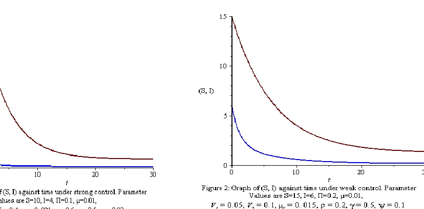
Figure 1 depicts a situation when there is strong control. With the assumed values stated under figure 1 together with 𝜋=0.1, 𝜀= 0.01, 𝛽1=0.03, 𝛽2=0.02, ℵ=0.04 and 𝛿=0.5, the reproduction number in equation
(16) is simulated to be 0.011 i.e𝑅0𝑞 = 0.011 <1 . The disease free equilibrium is globally asymptotically
stable under this condition. Figure 1 shows that over the time span of 30 days when 𝑅0𝑞 <1, the number of
susceptible (S) and infective (I) decreases significantly as the days of infection increase and the disease eventually disappears with time. Figure 1 is obtained from equation (5).
Similarly, using parameter values under figure 2 together with𝜋=0.2, 𝜀= 0.03, 𝛽1=0.045, 𝛽2=0.035, ℵ=0.06
and 𝛿=0.5 to simulate equation (16) then 𝑅0𝑞 = 3.232 >1 and the disease free equilibrium is unstable.
35
Moreover, by using parameter values under figure 3 together with 𝛽 =0.5, ℵ=0.4to simulate equation (17) then, 𝑅0 = 341.131 >1 and the disease free equilibrium is unstable. It is observed from figure 3 that during
the period of simulations the number of susceptible S and infectious I falls very slowly as the curves move away from the origin with larger number of infectious population at the end of the simulation which signals a major cholera tragedy in the population. Figure 3 is obtained from equations (1) – (4).
6.0 Conclusion
This work examined the global asymptotic stability of the two equilibrium states of a cholera model with prevention and control strategies. The DFE is globally asymptotically stable if 𝑅0𝑞<1 while the endemic
equilibrium is globally asymptotically stable if 𝑅0𝑞 >1. Graphical representations of the two cases i.e the
DFE and the EE are provided with separate cases of mild endemism and major endemism i.e 𝑅0𝑞 >1
and 𝑅0> 1. The graphs are used to illustrate the effect of strong control, weak control and no control on
the dynamics of cholera disease with reference to the existence of 𝑅0𝑞 <1, 𝑅0𝑞 >1 and 𝑅0> 1 .The results
obtained in this work strongly suggest that each community especially in less developed countries like Nigeria should be on red alert against the possibility of cholera outbreak. Besides, we find that to prevent and eliminate cholera in the population, there is a need to decrease the transmission rate and increase the treatment rate through adequate prevention and control measures. On that ground, relevant agencies should deem it fit to provide adequate enlightenment and sensitization to the general public on the need for environmental sanitation, personal hygiene and the dangers of land and water pollutants. Besides, provision of drinkable water and immunization are also necessary as all these will work together to reduce the parameters ℵ, 𝜀, 𝛽1 , 𝜇𝑐 , and𝛽2. Above all, immediate response to cholera outbreak by the Government,
health practitioners and the general public are capable of increasing the parameters 𝑣2 and 𝜌 and eventually
36
References
Bowon, S., Tewa, J. J., & Kamgang, J. C. (2011). Stability analysis of the transmission dynamics of tuberculosis model. World Journal of Modelling and Simulation, 7(2), 83-100.
Buonomo, B., & Lacitignola, D. (2010). Global stability for four dimensional epidemic models.
Note Mathematics, 30(2), 83-95.
Buonomo, B., & Vargas-De-Leone, C. (2013). Stability and bifurcation analysis of a vector-bias model of malaria transmission. Mathematical Biosciences, 242, 59-72.
Cheng, Y., Wang, J., & Yang, X. (2012). On the global stability of a generalised cholera epidemiological model. Journal of Biological Dynamics, 6(2), 1088-1094.
Codeco, C. T. (2001). Endemic and epidemic dynamics of cholera: The role of aquatic reservoir. BioMedcentral infectious diseases, 1(1), 1471-2334.
Fung, I. C-H.(2014). Cholera transmission dynamic models for public health practitioners. Fung Emerging themes in epidemiology. htpp://www.ete-online.com./content/11/1/1.
Hongwu Qin, Xiuqin Ma, Tutut Herawan, Jasni Mohamad Zain (2011). An adjustable approach to interval- valued intuitionistic fuzzy soft sets based decision making, Lecture Notes in Computer Science
(LNCS) Intelligent Information and Database System, Vol. 6592 (2011), pp.80-89. Springer Berlin/Heidelberg.
Santi Wulan Purnami, Jasni Mohamad Zain, Tutut Heriawan (2011). An alternative algorithm for classification large categorical dataset: k-mode clustering reduced support vector machine, International Journal of Database Theory and Application (IJDTA), Vol. 4, No. 1, pp. 19-29.
Shuai, Z., & van den Driessche, P. ( 2013). Global Stability of Infectious disease models using Lyapunov functions. SIAM Journal of Applied Mathematics, 74, 1513 – 1532.
Tian, J. P., Liao, S., & Wang, J. (2010). Dynamical analysis and control strategies in modelling cholera. Retrieved from: http://www.math.wm.edu/jptian/tain-liao-wang.
Tian, J. P., & Wang, J. (2011), Global Stability for Cholera Epidemic Models. Mathematical Biosciences 232, 31-41.