Time-frequency analysis based on wavelets for Hamiltonian systems

(1)

Hamiltonian Systems

Thesis by

Luz Vianey Vela-Arevalo

In Partial Fulfillment of the Requirements for the Degree of

Doctor of Philosophy

California Institute of Technology Pasadena, California

2002

(2)

c

° 2002

(3)

Acknowledgements

I would like to express my gratitude to those who contributed throughout all my years as a graduate student and, particularly, made this thesis possible.

I first would like to greatly thank my advisor Prof. Jerrold E. Marsden, for the most valuable academic and personal advising. His deep and insightful guidance was the best thing any grad student can hope for from an academic advisor. He exceeded by far any obligations that an advisor would have in providing support and I would like to express my gratitude for that.

My deepest thanks to my examination committee members: Emmanuel J. Candes, John Doyle, George Haller, Richard M. Murray and again Jerrold E. Marsden, first for accepting being part of the committee, and mainly for their very helpful and insightful comments during the revisions of the thesis and final defense. This is a good opportunity to acknowledge the advice of Joaqu´ın Delgado Fernández and Ernesto Pérez Chavela during my undergraduate and master’s work in the Universidad Autónoma Metropolitana-Iztapalapa. Thanks to them I became interested in dynamical systems in the first place, and I am very grateful for their guidance and friendship.

I would also like to thank Stephen Wiggins for his guidance in the initial steps of this work. I thank Laurent Wiesenfeld for interesting discussions during the year he spent as a visitor faculty at Caltech. I would like to express my gratitude to Turgay Uzer for numerous and fruitful discussions.

(4)

envi-ronment and meet many people during the time I was its president and organizer of Semana Latina.

I will never express enough gratitude to my parents Elodia and Francisco, my sister Christy, and my brothers Paco and Omahar, for their unconditional love, endless support and inspiration.

And most of all, I want to thank and dedicate this thesis to Thanos. His presence in my life has represented the most important motivation.

(5)

Time-Frequency Analysis Based on Wavelets for Hamiltonian Systems

by

Luz Vianey Vela-Arevalo

In Partial Fulfillment of the Requirements for the Degree of

Doctor of Philosophy

Abstract

In this work, we present the method of time-frequency analysis based on wavelets for Hamiltonian systems and demonstrate its applications and consequences in the general dynamics of higher dimensional systems.

By extracting instantaneous frequencies from the wavelet transform of numer-ical solutions, we can distinguish regular from chaotic motions, and characterize the global structure of the phase space. The method allows us to determine res-onance areas that persists even for high energy levels. We can also show how the existence of resonant motion affects the dynamics of the chaotic motion: we de-tect when chaotic trajectories are temporarily trapped around resonance areas, or undergo transitions between different resonances. This process is a good indicator of intrinsic transport in the phase space.

The method can be applied to a large class of systems, since it is not restricted to nearly integrable systems expressed in action-angle variables, which is the tra-ditional framework for the definition of frequencies.

(6)

We present three different applications of the method.

(7)

List of Figures

2.1 Density plot of the modulus of the wavelet transform of a function with linearly increasing frequency. Note that the ridge of the wavelet transform goes along the instantaneous frequency. . . 14 2.2 a) Analytic signal with variable phase and amplitude, and b)

mod-ulus of its wavelet transform. In c), we can see that the maximum of the modulus of the wavelet transform coincides with the instan-taneous frequency of the function defined as the derivative of the instantaneous phase. . . 31 2.3 a) Two frequency components with variable phase and amplitude,

and b) modulus of its wavelet transform. In c), we show how the instantaneous frequency is determined by the absolute maximum (in frequency) for each point in time. . . 32 2.4 Analyzing functions in a) the Gabor transform, and b) the wavelet

transform. The plots correspond to low frequency and high fre-quency. . . 34 3.1 Energy levels for a slice of the phase space corresponding to θ1 =

θ2 = θ3 = 0, projected onto the action plane (I1, I2), with I3 =

P ₋2(I1+I2), and P = 34.5. . . 41

(11)

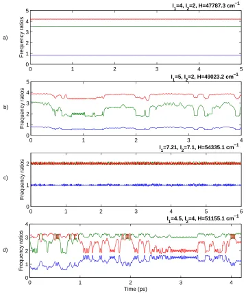
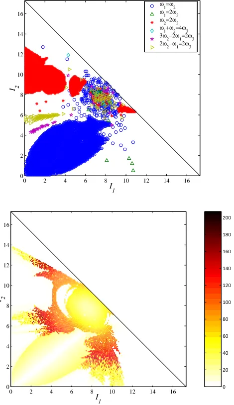
3.3 Time-frequency analysis for some trajectories of the Baggott Hamil-tonian, ω1/ω2 is blue, ω1/ω3 is green, and ω2/ω3 is red. a)

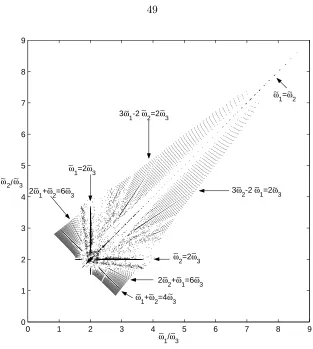
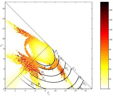
corre-sponds to a quasiperiodic trajectory, meanwhile b), c) and d) cor-respond to chaotic trajectories. . . 47 3.4 Arnol’d web of the Baggott Hamiltonian for P = 34.5. . . 49 3.5 Resonance channels. Stable two-tori are indicated in black circles. 51 3.6 Diffusion plot of the Baggott Hamiltonian. The points marked on

the energy contours correspond to the points in the Poincar´e sections of Figure 3.2. . . 52 3.7 One chaotic trajectory showing first low diffusion around the 2:1

resonance, and then wandering around the main resonance channels. See text for explanation. . . 57 3.8 Resonance channels and diffusion plot for the slice θ1 = π, θ2 =

θ3 = 0,I3 =P −2(I1+I2), P = 34.5. . . 59

3.9 Resonance channels and diffusion plot for the slice θ1 = θ2 = π,

θ3 = 0,I3 =P −2(I1+I2), P = 34.5. . . 60

3.10 Invariant curve Q1 ={N1 = 0}. Each curve corresponds to a

par-ticular value of the energy H0. . . 61

3.11 Intersection of the invariant surfacesQ2 ={N2=P/2}with a plane

ψ2 =constant, for different values of H0. . . 63

4.1 Hill’s region of the Sun-Jupiter system. Motion is possible in the interior region around the Sun, the Jupiter region, and the exterior region. . . 71 4.2 Poincar´e section corresponding to y = 0, vy > 0, and energy E =

−1.515. . . 72 4.3 Initial conditions for the frequency map: they are in the planex, vx

(12)

4.4 Results of time-frequency analysis: a) mean frequency (in ratio with the frequency of Jupiter), and b) the diffusion plot. . . 76 4.5 Examples of trajectories and the corresponding frequency evolution.

The orbits are represented in the inertial frame. The dotted line is the orbit of Jupiter. The frequency evolution is in ratio with the frequency of Jupiter. We have indicated the lines of the 2:3 and 3:2 resonances for reference. Note that the trajectories that go from the exterior region to the interior region “visit” the previous resonances. 77 4.6 Resonance trappings. The marks correspond to initial conditions

of orbits trapped in the resonances in the time interval indicated. Recall that the 3:2 resonance is in the interior region. Therefore trapping in this resonance occurs when the trajectory exchanges from the exterior to interior regions. . . 79 4.7 The large dots represent initial conditions of orbits that feature

rapid transition from the exterior to the interior regions, during the time interval indicated. The thick curve represents the first backward intersection of the stable manifold of the Lyapunov orbit around L2 with the Poincar´e section. The dots in the background

correspond to the Poincar´e map. . . 81 4.8 Percentage of trajectories that for the first time transition from the

exterior region to the interior region as a function of time; and similarly from the outer resonances (2:3, 1:2 and 3:5) to the inner resonance 3:2. . . 83 5.1 OCS molecule. . . 89 5.2 Contours of the potential energy function, for the collinear caseα=π. 91 5.3 Typical chaotic trajectory with large diffusion. The first plot shows

the frequency ratios, ω2/ω1 in blue, ω1/ω3 in green, and ω2/ω3 in

(13)

5.4 Mean frequenciesωe1,ωe2 andωe3 (a-c) and diffusion (d) for the total

integration time of 30 ps. . . 94 5.5 Resonance channels: Periodic and quasiperiodic trajectories with

resonant frequencies. We show the most important resonance junc-tions and single resonances. Representative trajectories very close to the periodic orbits in the resonance junctions are plotted. See text for more details. The trajectories were projected on the planes of motion (R1, P1), (R2, P2), (α, Pα). . . 97

5.6 Trajectory satisfying 4ω1 = ω2, ω1 = ω3 and ω2 = 4ω3 for 30 ps.

The assignment of colors is the same as in Figure 5.3. . . 98 5.7 Trajectory with large diffusion temporarily trapped in the resonance

junction ω1 =ω2 = 4ω3, and jumping close to the resonance

junc-tion 2ω1 = 3ω3 and ω2 = 3ω3. In b) we can observe how the

tra-jectory jumps almost instantaneously between the resonances. The assignment of colors is the same as in Figure 5.3. . . 101 5.8 Examples of resonance trappings. The assignment of colors is the

same as in Figure 5.3. . . 102 5.9 Resonance trappings for different intervals of time: a) 0 < t < .5,

b) 1 < t < 1.5 and c) 5 < t < 5.5 (ps). The arrow points towards initial conditions living in this resonance junction up to 30 ps. . . . 105 5.10 The first panel shows the percentage of trajectories that are trapped

in the resonance junctions of Figure 5.5 as a function of time. In the second panel, we consider only temporary trappings, i.e. trappings of chaotic trajectories. See text. . . 106 5.11 Chaotic trajectories trapped in a resonance for long periods of time,

(14)

List of Tables

(15)

Chapter 1 General Introduction

The coexistence of chaos and order is a common feature of nonintegrable Hamilto-nian systems. For systems of two degrees of freedom, it is possible to construct a two-dimensional Poincar´e map, where commonly we observe islands of quasiperi-odic motion surrounded by a chaotic ocean. However, the generalization of this picture beyond two degrees of freedom is far from being understood, in part for the lack of techniques of analysis available; but essentially for the different dynamical features of higher dimensional systems. For instance, in the case of three degrees of freedom, invariant tori are objects of dimension at most three in a five-dimensional energy surface; therefore, they are no more barriers in the phase space.

In this work, we propose a new method of time-frequency analysis based on wavelets. With this method, we generalize the notion of frequency map tradition-ally defined for completely or nearly integrable Hamiltonian systems. We are able to compute a frequency map for systems that are not nearly-integrable, or that are not given in action-angle coordinates.

(16)

resonance, providing a mechanism for intrinsic transport in the phase space. The method is successfully applied to a large variety of problems, ranging from molecular systems to celestial mechanics. In this work, we present a detailed analysis of two molecules, water and OCS; and the application to a comet cap-ture problem represented by the planar circular restricted three body problem in celestial mechanics.

The computation of frequencies from numerical solutions of dynamical sys-tems has been used as an analytical tool in fields as diverse as galactic dynam-ics [6, 7], chemical physdynam-ics [34], celestial mechandynam-ics [24] and molecular dynamdynam-ics [33, 51, 52, 30]. Since the existence of quasiperiodic solutions for integrable and nearly integrable systems is guaranteed by the KAM theorem [4, 8], the approxi-mation of the solutions by (truncated) Fourier series is justified for a large set of trajectories, that is, the quasiperiodic trajectories that remain on Diophantine tori. Therefore, this procedure calls for constructing an approximation of the solutions by trigonometric polynomials in terms of the nbasic frequencies of a system ofn

degrees of freedom.

We have extended this analysis to systems in which highly chaotic dynamics exists next to quasiperiodic trajectories. We use the method of time-frequency analysis based on wavelets to compute the evolution in time of the basic frequen-cies of the trajectories. This allows us to identify quasiperiodic trajectories with constant frequencies with respect to time; and chaotic trajectories featuring great time-variation of their frequencies.

We will argue that our method has several advantages over other available techniques for higher dimensional systems, specially with respect to the frequency analysis based of the Fourier transform that has been extensively used in Hamil-tonian systems.

(17)

advantage of the automatic localization in time and frequency that the wavelets provide, thereby avoiding the “averaged” results that Fourier analysis can give when applied to functions which are not quasiperiodic.

Time-frequency analysis based on wavelets turns out to improve the resolution of the time evolution of the fundamental frequencies when compared with Fourier-based methods. Indeed, our analysis has resulted in a number of surprising find-ings; e.g., we can observe how chaotic trajectories can be trapped temporarily in a single resonance or in resonance junctions. This is one of our main results.

As a further consequence of the superior accuracy of the time-evolution of the frequencies, we can determine exactly the time interval when a chaotic trajectory is temporarily trapped in a resonance, meaning that the trajectory remains close to a lower dimensional torus during that time-interval. When a resonance transition occurs, the trajectory has evolved from being trapped around one resonant torus to another one, indicating an exchange between different regions of the phase space. We use this fact to explain transport in phase space.

We believe that the main contribution of time-frequency analysis based on wavelets is that chaotic trajectories are included in the analysis besides the quasi-periodic trajectories. In this way, we can provide a detailed description of the global dynamics without any assumptions regarding the measure of the chaotic zones.

1.1 Organization of thesis

The thesis is organized in six chapters. The first chapter is a general introduction where the motivation and main results are presented.

In Chapter 2 we describe the necessary background in the definition of a more general frequency map for Hamiltonian systems. We also present the general theory for definition and extraction of time-varying frequencies and their use in analysis of Hamiltonian systems.

(18)

time-frequen-cy analysis based on wavelets. In Chapter 3, the classical version of the quantum Hamiltonian of the water molecule is analyzed. This is a three degrees of freedom (dof) system in action angle coordinates, that due to symmetries and a second integral of the motion, can be reduced to 2-dof.

In Chapter 4, the transport mechanism in the planar restricted three body problem is explained in terms of resonance transitions.

In Chapter 5, we describe the phase space dynamics of the 3-dof Hamiltonian for a vibrational model of the OCS molecule, in a highly excited state.

(19)

Chapter 2 Time-Frequency Analysis Based on Wavelets

for Hamiltonian Systems

2.1 Introduction

The purpose of this chapter is to describe the use of the wavelet transform in the definition and computation of a frequency map for a more general class of Hamilto-nian systems. The main idea of the method is to introduce the time variable in the analysis, and this is done by computing time-varying orinstantaneousfrequencies, extracted from the numerical solutions.

(20)

applicability of this concept in real signals such as numerical trajectories. The wavelet transform of analytic signals can be used to extract the instantaneous fre-quency of an analytic signal, this is discussed in Section 2.5. This algorithm is generalized to extract the instantaneous frequency from signals featuring oscilla-tory behavior. In Section 2.6, we point out that the case of multiple frequency components can be treated in a practical way since the formal definition of instan-taneous frequency does not apply. This will be important for Hamiltonian systems in which the coupling between dynamical variables produces the existence of two or more frequencies varying in time. Finally, in Section 2.7, we compare the method of time-frequency analysis based on wavelets with other available methods.

2.2 Frequency map in completely and nearly integrable

systems

2.2.1 Definition of the frequency map

The frequency map is traditionally defined in the context of completely integrable Hamiltonian systems, that is, systems for which there is a set of independent integrals of motion which are in involution, and the number of integrals is the same as the number of degrees of freedom. If this is the case, the Liouville-Arnol’d theorem [4, 8] assures that it is formally possible to find a canonical transformation that allows us to express the Hamiltonian system in action-angle variables in each bounded component of the constant energy manifold. Therefore, the frequency map is defined in these regions. Knowledge of the frequency map for such systems is sufficient to completely describe the dynamics.

Consider a completely integrable Hamiltonian system withndegrees of freedom expressed in action-angle coordinatesI, θ,

H(I, θ) =H0(I),

(21)

The equations of motion are given by

˙

Ik = 0,

˙

θk =

∂H0

∂Ik

(I) =:ωk(I). (2.1)

The solutions can be easily obtained as functions of time,

Ik(t) =Ik0,

θk(t) =ωk(I0)t+θ0k, k= 1, . . . , n.

Therefore, the motion takes place on a n-dimensional torus parameterized by the vectorI0. The trajectories are quasiperiodic functions in each of the planes of

motion, this is, the complex functions

zk(t) = q

2I0 k ei ωk(I

0₎_t₊_θ0

k

are quasiperiodic functions oft. The frequency map is defined as

I _→ω(I), (2.2)

and ω1, ω2,. . . , ωn are said to be the frequencies of the torus. If the frequency

map is invertible, we can use the frequencies ωk instead of the actions Ik as the

coordinates.

The frequencies determine completely the dynamics on the torus: if the fre-quencies are non-resonant, this is, if

m1ω1+m2ω2+· · ·+mnωn6= 0,

(22)

are dense on the torus. On the other hand, if an equation of the form

m1ω1+m2ω2+· · ·+mnωn= 0

is satisfied for some integer vector (m1, m2, . . . , mn) with not all the components

zero, then we call the torusresonantand in that case the trajectories lie on lower-dimensional tori, the dimension depending on the multiplicity of the resonance; this is, the dimension is the same as the dimension of the frequency module.

The definition of the frequency map (2.2) is basically attached to the repre-sentation in action-angle coordinates of a completely integrable system. This idea can be extended to any quasiperiodic solution, since it is possible to extract the frequency vector from any representation of a quasiperiodic solution. This is im-portant since the aim is to construct a frequency map (as in 2.2) independently of the coordinate representation of the system.

The method of frequency analysis calls for reversing the procedure: to extract the frequencies from the solutions, and then to obtain a characterization of the dynamics of the system based on the resonance relations of the frequencies.

Although the extraction of frequencies of quasiperiodic solutions is achieved with standard techniques of Fourier analysis, we will see that the generalization of the procedure to chaotic trajectories is not valid, even in the case of near-integrable systems.

In the following, we discuss the definition of quasiperiodic solutions and the use of Fourier analysis for the extraction of frequencies.

2.2.2 Quasiperiodic solutions

Consider a Hamiltonian system (not necessarily integrable) ofndegrees of freedom (n-dof), with Hamiltonian given by

(23)

wherexandyare general canonical position and momentum coordinates (and not action-angle coordinates). Assume that a quasiperiodic solution is known to exist, and is expressed as a complex variable zk(t) =xk(t) +i yk(t),k= 1, . . . , n.

In general, quasiperiodic functions are a special class of almost-periodic func-tions. A complex function f(t) is almost-periodic if it can be represented in the form

f(t) = ∞

X

j=0

cjei λjt (2.4)

where the coefficients cj _{are complex numbers. The numbers} _λj _{are called the}

frequencies of f. A vector function f = (f1,· · · , fn) is almost-periodic if all its

components are almost periodic.

The sub-class of quasiperiodic functions is characterized by expansions of the form (2.4) but in terms of a finite number of frequencies, i.e., they can be expressed as convergent Fourier series:

f(t) = X

m∈Zn

dmei m·ω t,

where m = (m1, . . . , mn) is an integer vector, ω = (ω1, ω2, . . . , ωn)∈Rn is called

the frequency vector, and m_·ω=m1ω1+· · ·+mnωn.

Almost-periodic solutions of an n-dof Hamiltonian system (2.3) are in fact quasiperiodic due to a result by Moser [37] showing that the number of basic fre-quencies is at mostn, the number of degrees of freedom. This is a consequence of the exactness of the symplectic form of the Hamiltonian system (see [37] and also [8], p. 125). Quasiperiodic solutions are characterized by the frequency vector, which is also associated to the n-dimensional invariant torus where the quasiperi-odic solution lies.

A quasiperiodic solution of (2.3) can therefore be expressed as

zk(t) = X

m∈Zn

dm_k ei m·ω t, k= 1, . . . , n. (2.5)

(24)

coordinate representation x0, y0 with frequency vector ω0, then there is a linear map L such that ω =Lω0_{, where} _L _{is a constant matrix with integer entries and} determinant _±1 [44].

Therefore, in the approximation of a quasiperiodic solution of (2.3) as

zk(t)≈ p X

j=0

cj_kei λjkt, k= 1, . . . , n, (2.6)

the numbersλj_kare integer linear combinations of the components of the frequency vector (ω1, . . . , ωn).

The computation of λj_k can be achieved using techniques of Fourier analysis, and from them we can extract the basic frequencies ω1, . . . , ωn and provide an

approximation of the solutions of the form (2.5). Once we know the frequencies associated to a particular quasiperiodic torus, we can describe the motion on the torus as resonant or non-resonant.

2.2.3 Computation of the frequency map in near integrable sys-tems using Fourier analysis

The procedure described above can be used for completely integrable systems, where all the bounded solutions are known to be quasiperiodic, and hence, Fourier analysis techniques apply. We can proceed in the same way for nearly integrable systems (this is, when a small perturbation is added), since the KAM theorem ensures the existence of quasiperiodic trajectories lying on slightly deformed in-variant tori with the same frequency vectors as in the unperturbed Hamiltonian, provided that Diophantine and non-degeneracy conditions are satisfied [1, 2, 8].

Laskar’s frequency analysis [25, 27, 26] provides an efficient algorithm for this case, by extending the Fourier basis to a more general set of complex exponentials. He proved that his method for approximating quasiperiodic solutions of nearly integrable systems provides the exact value of the frequencies with a certain con-vergence rate.

(25)

relies heavily on the fact that for systems that are integrable or near-integrable, there are many quasiperiodic trajectories for which the frequencies are well de-fined. An immediate concern is the treatment of chaotic trajectories generated by the perturbation. The generalization of the procedure to chaotic trajectories is frequently expressed as a negative statement: if we cannot assign frequencies to a particular solution, then the trajectory is deemed chaotic.

A common argument of Laskar [25], and Martenset al. [33], to justify the use of Fourier analysis in the case of chaotic trajectories is that for near-integrable systems, the behavior of its chaotic solutions is “regular enough” when viewed in short intervals of time. They assume that chaotic trajectories are close to quasiperi-odic locally, but this cannot be justified. The method we propose disregards this assumption.

2.3 Time-frequency analysis based on wavelets

As seen in Section 2.2, Fourier methods are justified for completely integrable systems, and even allows one to examine the behavior of many solutions of nearly integrable systems. However, chaotic trajectories in a very large class of non-integrable systems cannot be adequately examined.

Our main interest is to generalize the assignment of frequencies to solutions of Hamiltonian systems that feature oscillatory behavior. Although Fourier analysis provides a frequency representation of a time dependent signal, all Fourier methods require that the signal is periodic or quasiperiodic. Furthermore, this frequency representation does not reflect at all any change in time of the spectral information of the function. Therefore, frequency analysis based on the Fourier transform does not apply for systems that are not near integrable, even in principle.

(26)

Hamiltonian systems that are not nearly integrable, or that are not given in action-angle coordinates.

Advantages. The method we propose is time-frequency analysis based on

wave-lets. We compute the instantaneous frequency associated with time series repre-senting numerical solutions of the Hamiltonian system, producing the frequency evolution of the dynamical variables in the system. This will allow us to differen-tiate between regular and chaotic trajectories, since for quasiperiodic trajectories the frequencies are constant and coincide with the Fourier frequency. We can also identify resonance channels due to the good accuracy in the assignments of frequencies. Furthermore, the time evolution of the frequencies allows us to de-tect temporary resonance trapping of chaotic trajectories and their implications in transport in the phase space.

This methodology is inclusive, meaning that it can be applied on problems where Fourier methods apply, together with strongly chaotic systems.

2.3.1 Wavelet transform

An ideal method for analyzing functions that have time-varying frequencies is the

wavelet transform[12]. The wavelet transform by design provides good localization in both time and frequency. With this new methodology we will be able to define a frequency map for a large class of Hamiltonian systems, by the assignment of instantaneous frequencies to the trajectories.

The wavelet transform is defined in terms of a function ψ, called the mother wavelet, as

Lψf(a, b) =

1

√

a

Z ∞

−∞

f(t)ψ

µ

t₋b a

¶

dt. (2.7)

The function ψ _∈ L2(IR) must satisfy the admissibility condition 0 < cψ =

2πR_−∞∞ |ψb(_|_ωω_|)|2dω < _∞, where ψb is the Fourier transform of ψ; to be useful the mother wavelet must have compact support or decay rapidly to 0 for t_{→ ∞} and

t_{→ −∞}.

(27)

is the time parameter. The wavelet transform can be viewed as a time-frequency representation of a signal f in the following sense: If the wavelet ψ has compact support, the parameter b shifts the wavelets so that the local information of f

around the time t = b is contained in Lψf(a, b); the scale parameter a is

pro-portional to the inverse of the frequency; therefore, Lψf(a, b) gives the frequency

content of f over a small interval of time around t=b.

The wavelet transform (2.7) produces a complex surface as a function of the variables aand b. A common representation of this surface is a density plot of the modulus ofLψf(a, b), withbas the horizontal axis (time) andln(a) as the vertical

axis. However, since the frequency is proportional to the inverse of the scale (1/a), we opted for the frequency ω as the vertical axis.

2.3.2 A first example: the chirp

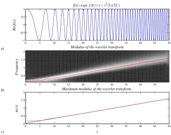
For motivation, and to show the capability of the wavelet transform to yield the variation in time of the frequency, consider the example given by a chirp; this is, a function with “increasing frequency.” In Figure 2.1 we present such example. In part a), the real part of a function with increasing frequency is represented, and in b) is the density plot of the modulus of its wavelet transform. We note that the density plot is “concentrated” or has the maximum along the line that corresponds to the time-varying frequency; this region is called the ridge of the wavelet transform.

In part c) of Figure 2.1, we plotted the frequency producing the maximum modulus as a function of time, and we observe that it coincides with the line that we expect to be the instantaneous frequency. Note that there is some discrepancy at the beginning and at the end of the time interval studied. This is caused by the finite interval considered in the analysis; this is, in the beginning and end of evolution, we do not possess enough information of the signal to perform the analysis. This is a normal limitation due to the finite time analysis.

(28)

a)

b)

c)

0 5 10 15 20 25 30 35 40 45 50

−1 −0.5 0 0.5 1

f(t)=exp( 2 π i ( t + t2/2 )/32 )

Re(f(t))

0 5 10 15 20 25 30 35 40 45

0.5 1 1.5 2

Frequency

Modulus of the wavelet transform

0 5 10 15 20 25 30 35 40 45 50

0 0.5 1 1.5 2

t

ω

(t)

Maximum modulus of the wavelet transform

Figure 2.1: Density plot of the modulus of the wavelet transform of a function with linearly increasing frequency. Note that the ridge of the wavelet transform goes along the instantaneous frequency.

time-frequency window in which the wavelet transform localizes the signal. Since our physical systems have bounded frequencies, this does not represent a problem in our analysis. This characteristic of the wavelet transform is reminiscent of the Heisenberg uncertainty principle: The localization in both time and frequency is limited. (See for instance [19]).

In the following, we describe the main properties of the wavelet transform in order to establish its convenience for time-frequency localization.

Zoom-in and zoom-out capabilities of the wavelet transform. We want

(29)

wide. The wavelet transform possesses this property, called the “zoom-in” and “zoom-out” capabilities. This fact will be clear from the determination of the time window and frequency window on which the wavelet transform is localized; for this we need to introduce some concepts.

The center and radius of the wavelet are defined (respectively) by

t∗ = 1

||ψ_||2 2

Z ∞

−∞

x_|ψ(x)_|2dx, and ∆ψ =

1

||ψ_||2

µZ ∞

−∞

(x₋t∗)2_|ψ(x)_|2dx

¶1/2

.

Assume ψ and its Fourier transform ψb are wavelets, with centers and radius

t∗, ω∗,∆ψ,∆ψb. Then, the wavelet transform 2.7 localizes the function within a

time window of the form

A= [b+at∗₋a∆ψ , b+at∗+a∆ψ].

Since the value of the frequency is proportional to 1/a, the time window automat-ically narrows for high frequency (asmall) and widens for low frequency (alarge); these are the zoom-in and zoom-out capabilities that we mentioned above.

Now, let η(ω) = ψb(ω+ω∗_{), the center of} _η _{is 0 and its radius is ∆}

b

ψ. Using

Parseval’s identity, we obtain that

Lψf(a, b) = √ a 2π Z ∞ −∞ b

f(t)eiωbη

µ

a(ω₋ω

∗

a )

¶

dω,

then the same quantityLψf(a, b) gives localized information of the spectrumfb(ω)

within a frequency window

B =

"

ω∗ a −

∆_ψ_b

a , ω∗

a +

∆_ψ_b

a

#

,

(with the exception of multiplication by √a/2π and a linear phase shift eiωb_).

(30)

Morlet-Grossman wavelet. The mother wavelet that we use throughout this work is the Morlet-Grossman wavelet [9], given by

ψ(t) = 1

σ√2π e

2πiλt_e−t2_/₂_σ2

.

The parameters λ and σ can be tuned to improve the resolution. This wavelet proved to be convenient for our computations, although the analysis can be done with other wavelets as well.

The simplest case. Consider a periodic functionf(t) =ei2πω0t_{, for which the}

wavelet transform can be obtained analytically as

Lψf(a, b) =

1

√

a

Z ∞

−∞

ei2πω0t_ψ µ

t₋b a

¶

dt

=√a

Z ∞

−∞

ei2πω0as_ei2πω0b_ψ₍_s₎_ds

=√a ei2πω0b_ψb₍_ω 0a),

where ψb is the Fourier transform of ψ. As we should expect the modulus of

Lψf(a, b) depends only on the scale a, and it is independent of the time variable

b.

Particularly for the Morlet-Grossman wavelet, the modulus of this transform is given by

η(a) =_|Lψf(a, b)|=√aψb(ω0a),

with ψb(ω) = e−2π2_σ2₍_ω₋_λ₎2

. η(a) has a global maximum, in other words, ψb is well localized in frequency. The maximum is at aω0 = 1₂

³

λ+qλ2₊ 1 2π2_σ2

´

.

Therefore, we can define the frequency variable (for the Morlet-Grossman wave-let) as

ω= 1 2a

Ã

λ+

r

λ2₊ 1

2π2_σ2 !

, (2.8)

and the value of the frequencyω0can be recovered from the scaleathat maximizes

(31)

be extended for functions that feature time-variation in frequency.

In the following, we will discuss the definition of instantaneous frequency and related concepts, and how they can be use to define a more general frequency map for Hamiltonian systems.

2.4 Instantaneous frequency

We want to use a definition of time-varying or instantaneous frequency that agrees with the intuitive notion of frequency as the “oscillation rate.” This definition must agree with the usual notion of Fourier frequency for signals with constant amplitude and frequency. In this way, periodic and quasiperiodic functions will retain their constant frequencies in the new analysis, and the frequency map will coincide with (2.2) for completely and nearly integrable Hamiltonian systems expressed in action-angle variables. Of the available definitions for instantaneous frequency, the one that satisfies this condition is based on the concept of analytic signal.

Assume that a complex function f(t) can be represented as a complex expo-nential with varying amplitude and phase,

f(t) =A(t)ei φ(t). (2.9)

Our intuition suggests that the frequency is given by time derivative of the phase:

ω(t) = 1 2πφ

0₍_t₎_.

(From now on we adopt the convention of the factor 2π in the definition of fre-quency). However, the representation (2.9) is not unique. To illustrate this with a simple example, consider

f(t) =A(t) cos(t),

(32)

the new function

˜

f(t) = (1/A˜)f(t).

Since _|f˜(t)_{| ≤}1, we can find ˜φ such that ˜f(t) = cos( ˜φ(t)). Therefore,

f(t) = ˜Acos( ˜φ(t))

is another representation of f which would have a different frequency.

The instantaneous frequency cannot be obtained from a particular representa-tion. We need to find a definition of instantaneous frequency that can be uniquely determined and that also corresponds to our physical intuition. Vakman [48] im-posed three conditions that instantaneous amplitude, phase and frequency should satisfy:

a) The amplitude is continuous and differentiable. This means that if the orig-inal function f changes slightly in amplitude, then the instantaneous ampli-tude should increase or decrease accordingly.

b) The phase is independent of scaling, and the amplitude is homogeneous; this is, if f(t) is replaced by cf(t), then the frequency does not change and the amplitude is scaled by c.

c) The constant amplitude and frequency of a simple sinusoid should retain their values.

Other authors have added new conditions, for instance Loughlin and Tracer [31] proposed that i) the instantaneous amplitude of bounded functions should be bounded, and ii) if the signal has bounded Fourier spectrum, the instantaneous frequency should have the same bounds.

(33)

2.4.1 Analytic signals

The most common definition of instantaneous frequency involves the concept of

analytic signal, introduced by Gabor [18] and Ville [50]. This definition includes the notion of Fourier frequency for periodic or quasiperiodic signals. The concept of analytic signal is based on the Hilbert transform.

Definition 1 A function f(t) = u(t) +i ν(t), expressed in terms of its real and

imaginary parts, is an analytic signal if

ν(t) =H u(t),

where

H u(t) =₋1

πP

Z ∞

−∞

u(η)

η₋tdη (2.10)

is the Hilbert transform ofu(t). Pdenotes the Cauchy principal value integral. We also say that u and ν form a Hilbert pair. The inverse of the Hilbert transform is given by

u(t) =H−1ν(t) = 1

πP

Z ∞

−∞

ν(η)

η₋tdη. (2.11)

We also say that the analytic signal associated to a real function u(t) is u(t) +

i Hu(t).

The following theorem provides three possible characterizations of analytic signals.

Theorem 1 Letf(t) =u(t) +i ν(t)be a piecewise continuous function with

piece-wise continuous derivative in any finite interval. Also, suppose f _∈ L1(R), and that f is bounded by decaying exponentials. The following are equivalent:

1. f is an analytic signal; i.e., ν(t) =H u(t).

2. The Fourier transform of f is one sided, i.e., it satisfies

b

(34)

3. f is obtained as the restriction to the real axis of a complex functionf(t+i τ)

that is analytic for τ _≥0; this is, f(t+i τ) =u(t, τ) +i ν(t, τ) is analytic in the complex upper half plane, and the signal satisfies

f(t) =u(t,0) +i ν(t,0), t_∈R.

The proof of this theorem contains a review of the mathematical concepts involved in the definition of instantaneous frequency, and can be found in the Appendix A.1. The concept of analytic signal is useful to define instantaneous frequency since for analytic functions the real and imaginary parts are uniquely defined; therefore, we are able to define the instantaneous phase and frequency in a unique way.

Definition 2 Let f(t) =u(t) +i ν(t) be an analytic signal, whereu and ν are the

real and imaginary parts respectively. The instantaneous phase of f is defined by

φ(t) = Arctanν(t)

u(t),

and the instantaneous frequency is the time derivative of the phase:

ω(t) = 1 2πφ

0₍_t₎_.

Identification of analytic signals. To determine if a function f(t) = u(t) +

i ν(t) is an analytic signal is not an easy task. Theorem 1 gives three possible characterizations of analytic signals; however, they are hard to use in practice and the analysis must be done numerically in most cases.

In general, functions arising from solutions of differential equations are not analytic signals. Most Hamiltonian systems have solutions that are not analytic in the upper half plane even if the Hamiltonian is analytic. Consider for instance the one-degree-of-freedom pendulum, which is of course integrable; its solutions can be expressed explicitly in terms of inverse elliptic functions that have a lattice of singularities in the complex plane.

(35)

Forstneric [16] has shown that the only Hamiltonian system inC2 of the form

H(z1, z2) =

1 2z

2

2+Q(z1) (2.12)

that has analytic solutions in the entire complex plane is forQquadratic. That is, if Qis not a quadratic function, every regular level set of (2.12) contains a point that flows to infinity in finite (complex) time.

In practical terms, the restriction of having a function of real time that has an analytic continuation to the upper half plane without any singularity is very strong.

The following examples illustrate some cases when analytic signals can be de-termined, and characterizations according to the definition or their spectral prop-erties.

Example 1. A trivial example of an analytic signal is the function f(t) =

exp(i2πω0t). To see this, note that the Fourier transform is one sided: F[f](ξ) =

δ(ω0−ξ); therefore, the imaginary part is the Hilbert transform of the real part,

H[cos(2πω0t)] = sin(2πω0t) and H−1[sin(2πω0t)] = cos(2πω0t),

and of course, the instantaneous frequency isω0.

This example shows that the definition of instantaneous frequency by means of analytic signals coincides with the definition of Fourier frequency for the case of constant frequencies. It is also clear that the Hilbert transform is linear and homogeneous, and that the instantaneous phase and frequency are independent of scaling. Therefore, this definition of instantaneous frequency satisfies the three conditions mentioned in the beginning of Section 2.4.

Example 2. u(t) and ˙u(t) (the derivative ofuwith respect tot) are not a Hilbert

(36)

Fourier transform of f,

F[f](ξ) =_bu(ξ) +ibu˙(ξ) =u_b(ξ) +i(2πiξ)_bu(ξ) = (1₋2πξ)u_b(ξ),

which is not one sided due to the fact thatu(t) is real and then its Fourier transform satisfiesub(₋ξ) =ub(ξ).

Example 3. Consider a function of the form A(t) exp(2πiω0t) with A(t) ≥ 0.

There is no a priori reason for this function to be an analytic signal. If this were the case, then we should have that

H[A(t) cos(2πω0t)] =A(t) sin(2πω0t) =A(t)H[cos(2πω0t)].

Let Ab(ξ) be the Fourier transform of A, then

F[A(t) exp(2πiω0t)] =Ab(ξ−ω0);

therefore,A(t) exp(2πiω0t) is an analytic signal if and only ifAb(ξ) = 0 for|ξ|> ω0.

This example can be seen as an application of the Bedrosian’s theorem that we enunciate in the following (for a proof see [21], p. 88).

Bedrosian’s Theorem. Letf, g _∈L1(R), such thatf ,bbg_∈L1(R) and

b

f(ξ) = 0, if_|ξ_|> ξ0, b

g(ξ) = 0, if_|ξ_{| ≤}ξ0,

then H[f(t)g(t)] =f(t)H[g(t)].

Consider again the function A(t) cos(2πω0t). IfAb(ξ) vanishes for |ξ|> ω0, we

can apply the Bedrosian’s theorem to obtain that

(37)

as we saw before.

Example 4. Bedrosian’s theorem gives the conditions on the Fourier transforms

of A(t) and cos[φ(t)] for which is valid

H[A(t) cosφ(t)] =A(t)H[cosφ(t)].

However, it is not clear that it should be H[cosφ(t)] = sinφ(t). In general this is not the case, an example is the following (taken from [40]):

Consider

x(t) = sin(2πBt)

2πBt cos(2πω0t),

whereω0 > B. Since|x(t)| ≤1, it is possible to introduce a functionφ(t) uniquely

defined such that 0_≤φ(t)_≤π and

x(t) = cosφ(t).

If it were true that H[cosφ(t)] = sinφ(t), then we should have

[x(t)]2+ [H x(t)]2= 1.

We will see that this is false. Since the Fourier transform of sin(2πBt)/(2πBt) is zero for _|ξ_|> B, we can apply Bedrosian’s theorem to get

H x(t) = sin(2πBt)

2πBt H[cos(2πω0t)] =

sin(2πBt)

2πBt sin(2πω0t),

and then

[x(t)]2+ [H x(t)]2=

µ

sin(2πBt) 2πBt

¶2

.

Example 5. We can apply the Bedrosian’s theorem to compute the Hilbert

transform ofA(t) cos(2πω0t+φ0) only if the Fourier transform ofA(t) vanishes for |ξ_{| ≥}ω0. Its analytic signal is in this case A(t) exp(i2πω0t+φ0). In general the

(38)

does not apply directly.

An asymptotic result can be obtained forω0 large [21]. Whenω0→ ∞we have

that

H[A(t) cos(2πω0t+φ0)] =A(t) sin(2πω0t+φ0)

for almost everyt.

Example 6. As we mentioned before, is not true in general thatH[cos(φ(t))] =

sin(φ(t)). If the function exp[iφ(t)] is an analytic signal, φ(t) must have the fol-lowing form [40]:

φ(t) =θ+ω0t+φb(t),

whereθ is arbitrary,ω0≥0 andφb(t) is the argument of a Blaschke functionb(t),

b(t) =

N Y

k=1

t₋zk

, Im(zk)>0;

i.e., φ(t) is the argument of a function of modulus 1 that has all its poles in the lower half complex plane.

A function with constant amplitude cexp[iφ(t)] is an analytic signal only if

φ(t) takes this particular form. This strong condition is very difficult to satisfy. In general, we should expect that analytic signals have the form A(t) exp[iφ(t)].

2.4.2 Asymptotic analytic signal

We have seen that the concept of analytic signal is very restrictive. In practice, we deal with functions that are close to an analytic signal. Delprat et al. [13] introduced the concept of asymptotic analytic signal.

Vaguely, a functionu(t) =A(t) cos(φ(t)) is called asymptotic analytic signal if its analytic signal associated,

Zu(t) =u(t) +i H[u(t)],

(39)

The following lemma shows that a function is an asymptotic analytic signal if the oscillations due to the term cos[φ(t)] are much more important than the variations of the modulus A(t). The proof can be found in the Appendix A.3, and it follows from the computation of the Hilbert transform using the stationary phase method (see Appendix A.2).

Lemma 1 Givenu(t) =A(t) cos[λφ(t)]withλlarge, the analytic signal associated

Zu(t) = [I+i H]u(t) satisfies

Zu(t) =A(t) exp[iλφ(t)] +O(λ−3/2).

This result is used in practice rather loosely, since in general there is not a parameterλcontrolling the rate of oscillation. However, we expect that functions with oscillatory behavior with a representation A(t) exp[iλφ(t)] are close enough to an analytic signal in such a way that the definition of instantaneous frequency applies.

2.5 Instantaneous frequency and the wavelet

trans-form

In the previous Section, we reviewed the definition of instantaneous frequency for analytic signals, and the difficulties to use it in practice since in general we deal with functions that are only close to an analytic signal.

In this Section, we study the relation of the wavelet transform with instan-taneous frequency of an analytic signal, and generalize this procedure towards numerical algorithms that allow us to extract time-varying frequencies.

All the arguments follow closely [13] and [9], and are explained here for com-pleteness.

(40)

waveletψ:

ψab(t) =

1

√

aψ

µ

t₋b a

¶

, b_∈R, a >0.

The coefficients of this expansion are given by the wavelet transform of f,

Lψf(a, b) = hf, ψabi =

1

√

a

Z ∞

−∞

f(t)ψ

µ

t₋b a

¶

dt.

Let f(t) = Af(t) exp[i φf(t)] be an analytic signal. If the wavelet ψ is an

analytic signal itself, and it is written in the form

ψ(t) =Aψ(t) exp[iφψ(t)],

then the wavelet transform coefficients can be computed as

Lψf(a, b) =

1

√

a

Z ∞

−∞

Mab(t) exp[iΦab(t)]dt, (2.13)

where

Mab=Af(t)Aψ µ

t₋b a

¶

,

Φab(t) =φf(t)−φψ µ

t₋b a

¶

.

In order to obtain an asymptotic expression for the integral in Equation (2.13), we note that if the integrand oscillates greatly due to the term exp[iΦab(t)], then the

functionMab(t) appears as constant and the contributions of successive oscillations

effectively cancel. However, if the phase Φab(t) is constant, i.e., there is a stationary

point, this effect is reduced. Therefore, the coefficients of the wavelet transform will “concentrate” around the stationary points.

Let t0 be a unique point such that Φ0ab(t0) = 0 and Φ00ab(t0) 6= 0. t0 is called

(41)

A.2) to obtain the expression,

Lψf(a, b)≈

1

√

af(t0)ψ

µ

t0−b

a

¶ s

2π

|Φ00_ab(t0)|

eisgnΦ00ab(t0)π/4. (2.14)

Note: t0 =t0(a, b). Then the equationt0(a, b) =bgives a curve in the time-scale

plane. This leads to the following definition:

Definition 3 The ridge of the wavelet transform is the collection of points for

which t0(a, b) =b.

From the equation Φ0_ab(t0) = 0, we have that

Φ0_ab(t0) =φ0f(t0)−

1

aφ

0

ψ µ

t0−b

a

¶

= 0, (2.15)

and then, by definition, the points on the ridge satisfy

a=:ar(b) =

φ0_ψ(0)

φ0_f(b).

Therefore, the instantaneous frequency φ0_f(b) of the function f can be obtained from this equation once we have determined the ridge of the wavelet transform.

2.5.1 Extraction of the ridge of the wavelet transform

(i_{) From the modulus of the wavelet transform.} _{In Figure 2.1 we showed}

with an example that the modulus wavelet transform has a maximum along the ridge. The ridge of the wavelet transform can be obtained by computing the maximum modulus of the wavelet transform (with respect to scale) for each point in time. Therefore, the maximum in scale for each time t=b corresponds to the instantaneous frequency of f, using the relation (2.8) (or an analogous one if a different mother wavelet is used).

(42)

(ii_{) From the phase of the wavelet transform.} _Delprat_{et al.} _{[13] described} an algorithm is to extract the ridges from the phase of the wavelet transform. This is explained in the following:

Define the phase of the wavelet transform of f (2.13) as

Ψ(a, b) = Arg(Lψf(a, b)).

From the asymptotic approximation in (2.14), we obtain

Ψ(a, b)_≈Φab(t0)±π

4.

Note that, from the definition of the ridge of the wavelet transform, t0 =

t0(a, b), i.e., Φab(t0) is a function of the variables a and b. Then, computing the

partial derivative with respect to b we have

∂Ψ

∂b ≈ ∂Φab

∂b

=∂

∂b

½

φf(t0(a, b))−φψ µ

t0(a, b)−b

a

¶¾

=φ0_f(t0)

∂t0

∂b −φ

0

ψ µ

t0−b

a

¶ Ã∂t0 ∂b −1

a

!

=

·

φ0_f(t0)−1

aφ

0

ψ µ

t0−b

a ¶¸ ∂t0 ∂b + 1 aφ 0 ψ µ

t0−b

a ¶ =1 aφ 0 ψ µ

t0−b

a

¶

.

(In the last step, the quantity in brackets is equal to zero due to Equation (2.15)).

Evaluating atb=b0 (and thent0(a, b0) =b0) we obtain

∂Ψ ∂b ¯ ¯ ¯ ¯

b=b0 ≈1_aφ0_ψ

µ

t0−b0

a

¶

=1

aφ

0

(43)

This equation provides an algorithm to extract the scalear(b0) that solves the

ridge equation t0(ar(b0), b0) = b0, for each time-value b0. The algorithm consists

of finding the fixed point athat solves the equation

a= φ 0

ψ(0)

∂bΨ(a, b)

,

for each b fixed. Therefore, given an initial approximation a0, we can produce a sequence of points aj+1 ₌ φ0ψ(0)

∂bΨ(aj,b) that converges to the solution a ∗_.

In this work we use a combination of the two approaches discussed above: the initial approximation is obtained from the maximum modulus of the wavelet transform evaluated on a series of test-frequencies, and then we use the fixed point algorithm to obtain an exact value of the frequency at each time.

2.6 Two or more frequency components

The definition of instantaneous frequency using the analytic signal has a phys-ical meaning only for signals that have a single frequency component varying in time (monochromatic). Although it seems intuitively plausible to consider functions with more than one frequency component varying in time, the defini-tion of instantaneous frequency is an ill posed problem in this case, as it has been pointed out often (see for instance [53]). In the case of two components

f(t) = a1expi φ1(t) +a2expi φ2(t), several physical restrictions lead to the

defi-nition of the instantaneous frequency as the average of the derivatives of the two phases, but only in the case that a1 = a2. Oliveira and Barroso [38] introduce

a heterodyne definition of frequency to obtain the average of the two frequencies agreeing with the definition of instantaneous frequency in the case a1 6=a2, and

also give conditions for the case ofn components.

(44)

trajectory, and we want to obtain the exact value of at least one of them. For us, the case of multicomponent signals can be addressed with a useful definition of instantaneous frequency, rather than a rigorous one.

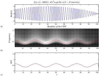
Consider the signalf(t) = (2₋.0005(t₋45)2_{) exp(2}_{π i}₍_.₅_t₊_._{6 sin(}_t/_{4))). This}

is a monochromatic function with variable phase and amplitude. We see that the variation of the amplitude is not as important as the oscillations due to the complex exponential; therefore, the definition of the instantaneous frequency as the derivative of the phase coincides with our intuition of what the frequency should be. This turns out to be correct since the function f, as a function of complex time t, is entire and therefore it satisfies the definition of analytic signal (Definition 1). In Figure 2.2 a) we plotted the real part of f, and the density plot of the modulus of its wavelet transform is represented in b); note that the maximum of this surface for each time value b corresponds to the instantaneous frequency at that given time, as it can be seen in c).

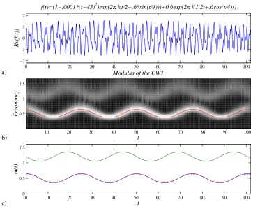
Consider now the function with two frequency components represented in Fig-ure 2.3. The function to analyze is f(t) = (1₋.0001(t₋45)2) exp(2π i(.5t+

.6 sin(t/4))) +.6 exp(2π i(1.2t+.6 cos(t/4))). Note in the density plot of the mod-ulus of the wavelet transform (Figure 2.3 b) that there are two ridges corresponding to two frequency components; the one with highest intensity corresponds to the component with higher amplitude (around frequency .5), and the band with less intensity corresponds to the component with lower amplitude (around frequency 1.2). This is, the modulus of the wavelet transform has two local maxima for each point in time. In this case, we consider as “the dominant frequency” the one with higher amplitude, corresponding to the absolute maximum. Hence, we define the instantaneous frequency as the one producing the absolute maximum of the modulus of the wavelet transform for each time.

(45)

a)

b)

c)

0 10 20 30 40 50 60 70 80 90 100

−2 −1 0 1 2

f(t)=(2−.0005(t−45)2)exp(2π i (t/2 + .6*sin(t/4)))

Re(f(t))

10 20 30 40 50 60 70 80 90 100

0.5 1 1.5

Modulus of the CWT

t

Frequency

0 10 20 30 40 50 60 70 80 90 100

0 0.5 1 1.5

t

ω

(t)

Figure 2.2: a) Analytic signal with variable phase and amplitude, and b) modulus of its wavelet transform. In c), we can see that the maximum of the modulus of the wavelet transform coincides with the instantaneous frequency of the function defined as the derivative of the instantaneous phase.

Due to the coupling terms, these time-series generally have several frequency com-ponents. Our aim is to identify n basic frequencies that describe quasiperiodic motions, and to determine how the frequencies vary in time for the case of chaotic trajectories. Therefore, in our heuristic solution for the multicomponent case, we consider only the absolute maximum of the modulus of the wavelet transform of

zk to obtain just one time-varying frequency, and disregard other local maxima.

(46)

a)

b)

c)

0 10 20 30 40 50 60 70 80 90 100

−2 −1 0 1 2

f(t)=(1−.0001*(t−45)2)exp(2π i(t/2+.6*sin(t/4)))+0.6exp(2π i(1.2t+.6cos(t/4)))

Re(f(t))

10 20 30 40 50 60 70 80 90 100

0.5 1 1.5

Modulus of the CWT

t

Frequency

0 10 20 30 40 50 60 70 80 90 100

0 0.5 1 1.5

t

ω

(t)

Figure 2.3: a) Two frequency components with variable phase and amplitude, and b) modulus of its wavelet transform. In c), we show how the instantaneous frequency is determined by the absolute maximum (in frequency) for each point in time.

as degrees-of-freedom of the system.

2.7 Other methods

(47)

The main advantage of our time-frequency analysis over other methods is that, besides the determination of quasiperiodic and chaotic trajectories, it provides de-tailed information regarding the order of the resonances in case of quasiperiodic trajectories; furthermore, the treatment of chaotic trajectories is done in a suit-able way and we are suit-able to detect resonance trappings and resonance transitions of chaotic trajectories. This information yields good picture of transport in the phase space. Also the applicability of time-frequency analysis is not restricted to near-integrable systems, but it can be used to analyze strongly non-integrable Hamiltonian systems.

Here, as a point of comparison, we outline the method of frequency analysis by Laskar, that can be seen as a special case of the Gabor transform. We refer the reader to [27, 25] for a detailed description and the numerical implementation of the method of Laskar; also see [26] for the analysis of the algorithm and its convergence.

2.7.1 Gabor transform

To include the time variation in the computation of frequency a second parameter is introduced in the Fourier transform, that will localize the spectral information around a given point in time. This results into theGabor transform[12, 9], in which the analyzing function is the usual complex exponential of the Fourier transform, multiplied by a Gaussian function that acts like a time-window:

F f(q, p) =

Z ∞

−∞

f(t)e−2πiqte−(t−p)2/2σ2dt

(48)

a) t

Re(g

q,p

)

g_q,p(t)=exp(2π i q t) exp(−(t−p)2/2σ2)

t

Re(g

q,p

)

b) t

Re(

ψa,b

)

ψ_a,b(t)=ψ((t−b)/a)

t

Re(

ψ a,b

)

Figure 2.4: Analyzing functions in a) the Gabor transform, and b) the wavelet transform. The plots correspond to low frequency and high frequency.

On the other hand and for comparison, in Figure 2.4 b) we represented the analyzing function in the wavelet transform for different frequencies. Note that the time window automatically contracts for higher frequencies and expands for low frequencies, according to the zoom-in and zoom-out capabilities of the wavelet transform described before. This is the main advantage of the wavelet transform over the Gabor transform, since this capability of adapting the time window to the frequency range produces better localization in time of the spectrum information of the signal.

Laskar’s frequency analysis

The method of frequency analysis by Laskar [27, 25] uses Fourier analysis to obtain approximations of quasiperiodic solutions by finite series of complex exponentials of the form PN_j₌₀ cje2πiωjt, cj ∈C.

(49)

consists of the numerical computation of the fundamental frequencyωk associated

to each degree of freedom zk = √2Ikeiθk of a given trajectory (z1, z2, . . . , zn)(t),

and of the approximation of the solution by an iterative scheme, giving

zk(t)≈c1e2πiωkt+ N X

j=2

cj_ke2πiωjkt.

If the given solution is quasiperiodic, a good approximation can be achieved and the value of the frequency vector ω = (ω1, . . . , ωn) is close to the actual rotation

vector of the trajectory. Thus, with this method we can determine and analyze quasiperiodic motions in the phase space. For instance one can identify resonant regions when we have a set of initial conditions for which their frequency vectorω

satisfies a resonance equation k_·ω= 0 for some integer vector k.

(50)

(51)

Chapter 3 Time-Frequency Analysis of Classical

Trajectories of the Water Molecule

Abstract

(52)

3.1 Introduction

The Baggott Hamiltonian is a quantum model of the water molecule which was originally developed by Baggott [5] using spectroscopic methods. It is a three-mode vibrational Hamiltonian featuring 1:1 Darling-Dennison resonance between the stretch modes and 2:1 Fermi resonance between the bend and stretches, where the symmetric x, K constraints have been relaxed to obtain better fitting to the experimental data. It has been used extensively in the literature in classical, semiclassical and quantum contexts. The same kind of model has been used for the description of triatomic symmetric molecules such as D2O, NO2, ClO2, O3

and H2S [32]. In these models there exists a constant of the motion known as

the Polyad number, which will translate into an independent first integral in the classical regime.

The classical version of the Baggott Hamiltonian is obtained using the Hei-senberg correspondence principle. It is a three degrees of freedom (dof) Hamilto-nian given in action-angle variables, and as the quantum version, contains 1:1 and 2:1 resonance couplings. The existence of the Polyad number allows the reduction of the system to 2-dof, and the global dynamics can be studied more easily.

In this work, we were interested in the case of Polyad number P=34.5, which corresponds to the quantum Polyad 16. This value is used in [22] to study the quantum-classical correspondence of highly exited states of the molecule.

In [22], a description of the classical phase space was given in terms of res-onant two-dimensional tori and resonance channels calculated with the Chirikov resonance analysis. This procedure uses the integrable limits of the Hamiltonian obtained when only one resonance coupling is considered. The location of the reso-nance channels was the basis for the classification of the eigenstates of the Baggott Hamiltonian.

(53)

of the Baggott Hamiltonian as a near integrable one is not so obvious.

We can also identify chaotic trajectories that are trapped temporarily around a resonant channel, suggesting the concept of time-varying resonances. This notion can explain how the energy of the system is distributed and how it is transported along the resonances during the evolution in time.

With the information of the resonances channels and the diffusion of the tra-jectories, we give a complete characterization of the dynamics in the phase space. The organization of this chapter is as follows: In Section 3.2 we present the Baggott Hamiltonian, and describe the reduction of the system to 2-dof. The time-frequency analysis based on wavelets was used to analyze the classical trajectories of this system; this is presented in Section 3.3 together with the description of how the resonance structures determine the dynamics of the system. We also identify the chaotic zones in the phase space by numerically computing the diffusion of the system. The conclusion is found in Section 3.4. In the Appendix A.5, we describe the transformations to obtain the 2-dof Baggott Hamiltonian.

3.2 Baggott Hamiltonian

The classical version of the quantum Hamiltonian for the water molecule by Bag-gott [5] is given by

H =H0+H1:1+H2:2+H12:1+H22:1, (3.1)

H0 =Ωs(I1+I2) + ΩbI3+αs(I12+I22) +αbI32+εssI1I2+εsbI3(I1+I2),

H1:1 =(β12+λ0(I1+I2) +λ00I3)(I1I2)1/2cos(θ1−θ2),

H2:2 =β22I1I2cos 2(θ1−θ2),

H₁2:1 =βsb(I1I32)1/2cos(θ1−2θ3),

(54)

where (I1, I2, I3, θ1, θ2, θ3) are action-angle coordinates.

The Baggott Hamiltonian is a three-degree-of-freedom (dof) system exhibiting 2:1 resonance between the bend and stretch modes, and 1:1 and 2:2 resonances between the two stretch modes. There is a permutation symmetry between the indices 1 and 2, and also note that the Hamiltonian is not differentiable atI1= 0 or

I2 = 0. The values of the parameters are obtained to fit the experimental spectra.

We used here the notation in [22]. See Table 3.1.

¯ ¯ ¯ ¯ ¯ ¯ ¯ ¯ ¯ ¯ ¯ ¯ ¯ ¯ ¯ ¯ ¯ ¯ ¯ ¯ ¯ ¯ ¯ ¯ ¯ ¯ ¯ ¯ ¯ ¯ ¯ ¯ ¯ ¯ ¯ ¯ ¯ ¯

Ωs 3885.57 (cm−1)

Ωb 1651.72

αs −81.99

αb −18.91

εss −12.17

εsb −19.12

β12 −112.96

λ0 6.04

λ00 ₋0.16

β22 −1.82

βsb 18.79

¯ ¯ ¯ ¯ ¯ ¯ ¯ ¯ ¯ ¯ ¯ ¯ ¯ ¯ ¯ ¯ ¯ ¯ ¯ ¯ ¯ ¯ ¯ ¯ ¯ ¯ ¯ ¯ ¯ ¯ ¯ ¯ ¯ ¯ ¯ ¯ ¯ ¯

Table 3.1: Parameters of the Baggott Hamiltonian.

The system possesses a first integral which is the classical expression of the quantum Polyad number of the system. It is given by

P = 2(I1+I2) +I3. (3.2)

This constant of motionP is related to the quantum PolyadPbyP = 2P+5/2 [22]. Equation (3.2) implies that the values of the actions are bounded: 0< I1 < P/2,

(55)

2 4 6 8 10 12 14 16 2

4 6 8 10 12 14 16

I

1

I 2

36000 40000 44000 48000 52000 56000

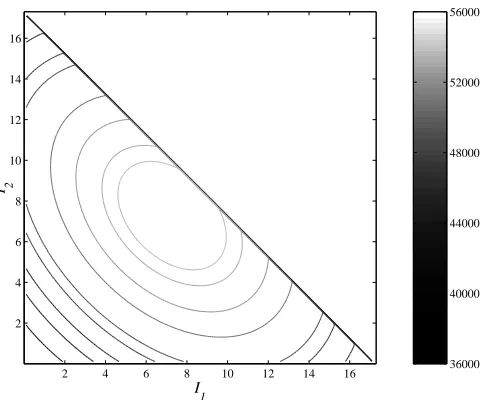
Figure 3.1: Energy levels for a slice of the phase space corresponding toθ1=θ2 =

θ3 = 0, projected onto the action plane (I1, I2), with I3 = P −2(I1+I2), and

P = 34.5.

In this work, we study the Polyad number P = 34.5, that corresponds to the quantum Polyad number P = 16. This is the same value used in [22] to study highly excited states of the molecule. We will use time-frequency analysis based on wavelets to give a more accurate and complete characterization of the phase space for this Polyad number.

Taking the angles θ1 = θ2 = θ3 = 0, the intersection of the energy surfaces

H =H0 with the planeP = 34.5 can be drawn as contours projected to the plane

I1, I2, since I3 is obtained from Equation (3.2). These contours are represented in

Figure 3.1.

Equation (3.2) will allow us to reduce the Baggott Hamiltonian to a 2-dof system. Via successive canonical transformations we obtain first the Hamiltonian in normal coordinates, and then a system in action-angle variables (N1, N2, N3,

ψ1, ψ2, ψ3) for which the third action satisfies