Accurate, fast and stable denoising source
separation algorithms
Harri Valpola1,2?and Jaakko S¨arel¨a2??
1
Artificial Intelligence Laboratory, University of Zurich Andreasstrasse 15, 8050 Zurich, Switzerland
2
Neural Networks Research Centre, Helsinki University of Technology P.O.Box 5400, FI-02015 HUT, Espoo, Finland
Abstract. Denoising source separation is a recently introduced frame-work for building source separation algorithms around denoising pro-cedures. Two developments are reported here. First, a new scheme for accelerating and stabilising convergence by controlling step sizes is in-troduced. Second, a novel signal-variance based denoising function is proposed. Estimates of variances of different source are whitened which actively promotes separation of sources. Experiments with artificial data and real magnetoencephalograms demonstrate that the developed algo-rithms are accurate, fast and stable.
1
Introduction
In denoising source separation (DSS) framework [1], separation algorithms are built around a denoising function. This makes it easy to tailor source separation algorithms for the task at hand. Good denoisings usually result in fast and accurate algorithms. Furthermore, explicit objective function is not needed, in contrast to most existing source separation algorithms.
Here we report further developments of two aspects. First, we introduce a new method for stabilising and accelerating convergence which is inspired by predic-tive controllers. Second, we develop further the signal-variance-based denoising principles. The resulting algorithms yield good results in terms of signal-to-noise ratio (SNR) and exhibit fast and stable convergence.
2
Source separation by denoising
Consider a linear instantaneous mixing of sources:
X=AS+ν, (1)
?
Funded by the European Commission, under the project ADAPT (IST-2001-37173) and by the Academy of Finland, under the project New information processing principles.
??
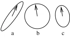
a b c
Fig. 1.a) Original data set , b) after sphering and c) after denoising. After these steps, the projection yielding the best signal-to-noise ratio, denoted by arrow, can be obtained by simple correlation-based learning.
where theN×T matrixSare the sources, theM×T matrixXare the observa-tions and there is noiseν. If the sources are assumed Gaussian, this is a general, linear factor analysis model with rotational invariance.
DSS, as many other computationally efficient ICA algorithms, resorts to sphering. In the case of DSS, the main reason is that after sphering, denois-ing combined with simple correlation based estimation akin to Hebbian learndenois-ing (on-line) or power method (batch) is able to retrieve the signal with the highest SNR. Here SNR is implicitly defined by the denoising. The effect of sphering and subsequent denoising is depicted in Fig. 1.
Assuming thatXis already sphered and f(s) is the denoising procedure, a simple DSS algorithm can be written as follows:
s=wTX (2)
s+=f(s) (3)
w+=Xs+T (4)
wnew= orth(w+), (5)
where s is the source estimate (a row vector), s+ is the denoised source
esti-mate, wis the previous weight vector (a column vector),w+ is the new weight
vector before and wnew after orthonormalisation (e.g., deflatory or symmetric
orthogonalisation as in FastICA [2]).
Note that ifXwere not sphered and no denoising were applied, i.e.,f(s) =s, the above equations would describe the power method for computing the princi-pal eigenvector. WhenXis sphered, all eigenvalues are equal to one and without denoising the solution is degenerate, i.e., any unit vector w is a fixed point of the iterations. This shows that for sphered X, even the slightest denoisingf(s) can determine the convergence point.
It is possible to begin with an objective functiong(s) in which case the de-noising can be chosen1 to be the gradient:f(s) =∇g(s). In practice, denoising
functions can easily be designed without explicitly starting from objective func-tions. They often work exceedingly well and good denoisings result in fast and accurate algorithms.
3
Accelerating and stabilising convergence by spectral
shift and adaptation of learning rate
If the denoising function is not able to reduce noise significantly more than signal, the basic DSS iterations (2)–(5) may converge slowly. This is closely related to the fact that power method converges slowly if the largest eigenvalue is only slightly larger than the next largest. Consequently, convergence in DSS can be accelerated in a very similar manner as in power method.
A well-known speedup for power method is spectral shift. It is based on modifying an iteration of the form w+ = Aw into w+ = Aw+βw. In the original iteration, it holdsw+=λwat the fixed points and consequentlyw+= (λ+β)w after the modification. The fixed points remain the same but the eigenvaluesλare shifted byβ, hence the name spectral shift.
If all eigenvalues are large and their differences are small, convergence can be greatly accelerated by usingβwhich is negative and whose absolute value is close to the second largest eigenvalue. On the other hand, power method converges to the eigenvector that corresponds to the eigenvalue having the largest absolute value. This means that instead of finding the principal component, the minor component is obtained with negative enoughβ.
In DSS, (3) can be modified into
s+=α(s)f(s) +β(s)s (6)
without changing the fixed points as long asα(s) andβ(s) are scalar functions. Sinceα(s) only scales the source estimate, from now on we assume α(s) = 1.
In DSS,s+sT/T plays the role of the eigenvalue [1]. Since Gaussian signals are the least desirable ones in source separation, a reasonable choice forβ is the one that shifts the eigenvalue of Gaussian signals to zero:
β =E{f(ν)νT/T}, (7)
whereν is a normally distributed signal.
It is interesting to note that the fixed-point equation of FastICA [2] can be interpreted within this framework although normally the speedup used in FastICA is justified as an approximation to Netwon’s method. In [1], it was shown that ifβ(s) is based on a linearisation off(s) around the current source estimates, the spectral shift (7) will be
β(s) =−trJ(s)/T , (8)
1
which is identical to the one used in FastICA. HereJ(s) is the Jacobian off(s). Interpreting the speedup as a spectral shift corresponding to Gaussian noise gives an intuitive explanation to why FastICA is able to extract both super- and sub-Gaussian signals with the same nonlinearity: power-method-like iterations converge to the eigenvector whose eigenvalue has the largest magnitude. The sign of the eigenvalue is different depending on whether the component is super-or sub-Gaussian but the magnitude increases when moving away from Gaussian signal whose eigenvalue has been shifted to zero.
In general, iterations converge faster with the FastICA-type spectral shift (8) than with the global Gaussian approximation (7) but the latter has the benefit that no gradients need to be computed. This is important when the denoising is defined by a complex nonlinear procedure such as median filtering.
Neither of the spectral shifts, (7) or (8), always results in stable or fast con-vergence. Sometimes the spectral shift is too large, which due to the nonlinear-ity of denoising typically leads to oscillatory behaviour: the iteration oscillates between two weight values. Some other times the spectral shift is too modest leading to slow convergence characterised by small changes of w in the same direction during several iterations.
For this reason, we have suggested a simple stabilisation rule [1]: instead of updating wintownew defined by (5), it is updated into
wadapted= orth(w+γ∆w) (9)
∆w=wnew−w, (10)
whereγ is the step size. Originallyγ= 1, but if the consecutive steps are taken in nearly opposite directions, i.e., the angle between ∆w and ∆wold is greater
than 179◦, then γ = 0.5 for the rest of the iterations. There exist a stabilised version of FastICA as well [2] and a similar procedure has been used in practice. The above modification is able to stabilise convergence in case of oscillations but sometimes the spectral shift is too small and then an increase in step size would be appropriate, i.e.,γ >1. We propose a simple rule for adaptingγwhich is inspired by predictive controllers used in robotics: a simple but slow and possi-bly unstable reactive controller is used for teaching a new, predictive controller. Usually stable and rapid convergence are difficult to achieve simultaneously, but in this setup the new controller can be both faster and stabler.
Translated in our problem, the old slow and unstable controller is the weight modification rule which proposes a modification of weight according to (10). The new controller is implemented by (9), i.e., it modifies the step size. The new controller tries to do immediately what the old controller would do in the future. The step at the previous time instant was apparently optimal if the step proposed at this time instant is orthogonal with it. If not, γ should have been different and, assuming that the optimalγ is constant, the gamma used at this time step should be
γnew=γold+∆woldT ∆w/||∆wold||2. (11)
The above adaptation ofγhas turned out to be very useful and it can both stabilise and accelerate convergence. According to (11), γ keeps increasing as long as the steps are taken to the same direction and decreases if they are taken backwards.
4
Denoising based on estimated signal variance
Several denoising procedures based on masking the source estimate were pro-posed in [1]. The basic idea is to multiply the source estimate by a positive envelope, a mask which has low values when SNR is low and vice versa. Depend-ing on how the mask is computed, several types of prior information about the sources can be used for separation.
A simple and well-founded mask can be obtained from the maximum-a-posteriori (MAP) estimate. Assuming that the signals are Gaussian with chang-ing varianceσ2
s(t) (for related methods, see, e.g., [3]) and additive Gaussian noise
σ2
n, the MAP estimate of the signal is
s+(t) =s(t) σ
2
s(t)
σ2 tot(t)
, (12)
where σ2
tot(t) =σs2(t) +σ2n(t) is the total variance of the observation. Masking then boils down to estimatingσ2
s(t) andσ2tot(t) from the observations.
A na¨ıve estimate of the signal variance isσ2
s(t)≈s
2(t). It can be improved
by low-pass filtering in time, e.g., by convolving with a Gaussian kernel. Simple estimation of the baseline noise-levelσ2
n was suggested in [1] resulting in a sim-ple DSS algorithm. However, from the viewpoint of the estimated signal, other signals should be treated as noise. DSS algorithm using the above approximation separates easily the signal subspace from noise but the separation in the signal subspace is slow and may even fail. In [1], this was solved by usingσ2µ
s (t) with
µ >1 in (12). This way the mask does not saturate so quickly for large signal variances, giving competitive edge to the source which is strongest. A close con-nection to the familiar tanh-nonlinearity was shown: f(s) =s−tanhshas the same fixed points asf(s) = tanhsbut the former can be interpreted assmasked by a slowly saturating envelope.
In this paper, we propose a new and better founded solution to the sepa-ration problem. One can simply whiten the estimated total variance σtot(t) by
a symmetric whitening matrix. This bares resemblance to proposals of the role of divisive normalisation on cortex [4] and to the classical ICA-method called JADE [5]. Whitening naturally requires that all sources are estimated simul-taneously and deflation approach is thus not applicable. The total variance is obtained by smoothing s2(t) as described above. We obtain σ2
s(t) by taking the positive part of the whitened σ2
tot(t). Whitening here includes removing the
179−rule predictive rule 0
100 200 400 600
iterations
a: gamma update no shift FastICA fixed shift
whiten var smooth tanh tanh 0
2 4 6 8
SNR / dB
b: denoising function
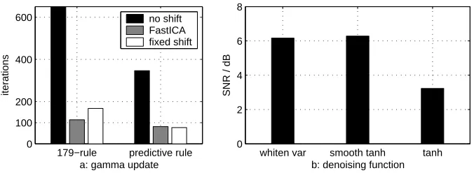
Fig. 2.Speedup tests. a) Effects of spectral shift and step-size adaptation on conver-gence speed. The leftmost bar not fully shown. b) Average SNRs for different denoising functions: variance whitening and tanh with and without smoothing.
5
Experiments
In this section, we show that the developed algorithms are fast, stable, accurate and produce meaningful results. First, in Sec. 5.1, we demonstrate the different spectral shifts and step-size adaptation. Then the accuracy of different denoising algorithms is tested with artificial data (Sec. 5.2). Finally, we demonstrate the separation capability and convergence speed of the variance-based-denoising in real MEG data (Sec. 5.3).
5.1 Speedup comparison
In Sec. 3, we reviewed two spectral shifts that can accelerate convergence in DSS algorithms. Later in the section, we proposed two additional methods to adapt these spectral shifts to increase stability. In this section, we compare these adaptive-spectral-shift methods together with the stability improvements in de-flatory separation. The data consists of M = 50 channels and T = 8192 time samples of rhythmic magnetoencephalograms (MEG) [6, 1]. The data was pre-processed as in [1] to enhance weak phenomena. Simple f(s) = s−tanhs was used as the denoising function. DSS was run to extract 30 components from this data and average number of iterations was calculated. To be fair for all the meth-ods, each of them was run until convergence, where the angle between old and new projection vectors (w andwnew) was less than 0.0001◦. We then measured
the number of iterations that had takenwwithin 0.1◦ of the final solution. The results are shown in Fig. 2a. Both types of spectral shift andγ adap-tation always accelerated convergence. Convergence without any speedups took on average more than 1500 iterations. Withoutγ adaptation, the FastICA-type scheme (8) converged faster on average than the fixed-shift scheme (7), but γ
5.2 Comparison of denoising functions
We next compare DSS schemes based on source-variance estimates to the clas-sical tanh-based approach in symmetrical separation of artificial signals. The signals were generated as follows. First, six signals were generated by modulat-ing Gaussian noise with slowly changmodulat-ing envelope. Then the signals were divided into two subspaces, three signals in each. In each of the subspaces, the signals were modulated by another envelope common to all the signals in the subspace. The common envelopes of the subspaces were stronger than the individual en-velopes of the sources. Finally, the unit-variance signals were mixed linearly (withM =N). Mixing coefficients were sampled from normal distribution and Gaussian noise with varianceσ2
ν = 0.09 was added.
One hundred different data sets were generated and DSS was used to separate the sources with three different denoising functions. Two methods were based on smoothed estimate of source variance. Either the whitening scheme described in Sec. 4 or tanh-based scheme were used in order to promote separation, the tanh-mask being 1−tanh[σtot(t)]/σtot(t). Ifσ2tot(t) =s
2(t), this reduces to the
popular tanh-nonlinearity. With these methods, spectral shift was computed by assuming that the mask does not significantly depend on any individual source value, i.e.−β equals to the average of elements of the mask. The third method was the popular tanh-nonlinearity with FastICA-type spectral shift. The step size was adapted by the 179-rule.
As before, the algorithms were run until convergence. The average SNRs of the separation over the one hundred runs are shown in Fig. 2b. Smoothing the variance estimate clearly improves the SNR with tanh-nonlinearity. Variance whitening achieved comparable SNR but used significantly less iterations.
5.3 MEG signal separation
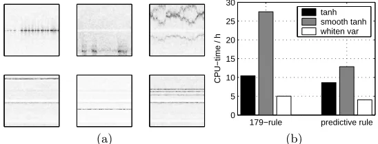
Finally, we used the DSS algorithms and acceleration methods studied in the previous sections to separate sources from rhythmic MEG data. The whole data set (M = 122 andT = 65536) was used and 30 components were extracted using the same denoising functions as in the previous section. Both the 179-rule and the predictive rule (11) were tested. The number of iterations was taken to be the limit where the projection vector w of the slowest converging component reaches 0.1◦ of the final projection. Enhanced spectrograms of some interesting components extracted by the variance-whitening DSS are depicted in Fig. 3a.
179−rule predictive rule 0
5 10 15 20 25 30
CPU−time / h
tanh smooth tanh whiten var
(a) (b)
Fig. 3. a) Spectrograms of some of the sources separated using variance whitening. Time on the horizontal and frequency on the vertical axis. b) Used processing time for different denoising functions and step sizes.
on the denoising function. Tanh-nonlinearity with smoothed variance estimate used a fixed spectral shift and benefitted more from adaptation of γ than the plain tanh-nonlinearity with FastICA-type spectral shift.
6
Conclusion
DSS framework offers a sound basis for developing simple but efficient and accu-rate source separation algorithms. We proposed a method for stabilising and ac-celerating convergence and showed that convergence is faster than with FastICA. Additional benefit is that gradient of the nonlinearity is not needed. We also proposed a new denoising procedure which was justified as the MAP-estimate of signals with changing variance. Denoising which makes use of non-stationarity of variance was shown to yield better results than the popular tanh-nonlinearity as measured by SNR in the artificially generated data. The variance-whitening DSS also extracted cleaner signals in MEG data, while the tanh-nonlinearity had difficulties with some weak but clear phenomena. Whitening the estimated variances of different sources significantly improved convergence.
References
1. S¨arel¨a, J., Valpola, H.: Denoising source separation. Submitted to a journal (2004) Available at Cogprintshttp://cogprints.ecs.soton.ac.uk/archive/00003493/. 2. Hyv¨arinen, A.: Fast and robust fixed-point algorithms for independent component
analysis. IEEE Trans. on Neural Networks10(1999) 626–634
3. Matsuoka, K., Ohya, M., Kawamoto, M.: A neural net for blind separation of nonstationary signals. Neural Networks8(1995) 411–419
4. Schwartz, O., Simoncelli, E.P.: Natural signal statistics and sensory gain control. Nature Neuroscience4(2001) 819 – 825
5. Cardoso, J.F.: High-order contrasts for independent component analysis. Neural computation11(1999) 157 – 192