Data Driven Analytical Modeling of Power Transformers

(1)

Article

Data Driven Analytical Modeling of

Power Transformers

Jyrki Penttonen 1,2,* and Matti Lehtonen 1

1_{Department of Electrical engineering, Aalto University, Otakaari 5, 02150 Espoo, Finland;}

[email protected]

2 _{Vensum Ltd., Pohjoisranta 8 E 116, 00170 Helsinki, Finland}

* Correspondence: [email protected]; Tel.: +358 45 6412938

Abstract: In power systems there are complex transformer structures, whose accurate analysis is not possible using the techniques available today. This paper presents a systematic data driven analysis method for coupled inductors of arbitrary complexity. The method first establishes a winding matrix N mapping the windings to the limbs of the transformer. A permeance matrix P is created from the reluctance network of the magnetic core. A generalized inductance matrix L mapping currents in the transformer windings to the induced voltages is generated based on the winding (N) and permeance (P) matrices. The inductance matrix representation of a coupled inductor is then transformed to an admittance matrix, which can be integrated to the nodal analysis of the electrical circuit surrounding the coupled inductor. The method presented is validated by simulations with real transformer structures using electromagnetic transient program (EMTP/ATP).

Keywords: power transformer; coupled inductor; electro-magnetic modeling

1. Introduction

1.1 Survey of known power transformer analysis methods

Transformer structures of today are getting more and more complex and there is a need to come up with a more systematic treatment of coupled inductors so, that the dynamics of them can be modeled effectively with electromagnetic transient programs such EMTP/ATP or Spice. Some of the hard problems the currently known transformer analysis methods are not able to deal with effectively are:

• Asymmetric nature of the magnetic core (eg. where the reluctances of individual limbs vary): in [1] there is an analysis of the three limb three phase transformer, when the different limbs have different reluctancies thus creating asymmetry. The method is hard to generalize as a number of assumptions have to be made during the analysis and the method is different for each different vector group.

• Integration with the surrounding electrical circuits in a systematic way: in [2] there is a

description of a method to analyze multiterminal three phase transformer in which there is an attempt to use matrices to represent the transformer winding structures. While this method is usefull, it cannot be generalized to complex transformers and electrical network connections.

• Complex multi limb structures: in [3-7] there are specific analysis of typical power transformer structures (3 phase, 3 or 5 limbs, symmetric/asymmetric). These methods are not suitable for more complex coupled inductors.

• Method presented in [8] builds matrices to represent the transformer structure, but it only

applies to three phase transformers and cannot be generalized.

(2)

One way for more accurate analytical treatment of leakage fluxes power transformer cores means, that the amount of magnetic paths in the magnetic core increases as one physical limb is broken down to a number of magnetic paths corresponding to a part of the limb and leakage magnetic path around it [10]. This means, that the magnetic model becomes intractable for the traditional methods designed for simpler three of five limb core structures.

In summary: most of the currently known methods for power transformer analysis are focused on analyzing transformers for predefined core structures (typically 3 limbs or 5 limbs) and with certain vector groups. If the core structure changes a new method is required and if the vector group changes, another change of method is required. Furthermore, when the core and winding structures get more complicated, for example when modeling core with reluctance networks involving leakage fluxes, there is no straightforward analysis method. When power transformer is analyzed in fundamental frequency, leakage fluxes and core asymmetries may not play a major role, but when analyzing transformer performance under fast transients, more accurate modeling becomes crucial.

2. Objectives of the work in this paper

To address the shortcomings of current power transformer analysis, as described above, this work provides a systematic treatment of coupled inductors so, that any power transformer core structure, vector group or surrounding electrical network can be modeled without changes needed in the analysis method. The proposed method is data driven: transformer core is modeled by a numerical matrix representing its reluctance network and the windings are modeled as another numerical matrix. Thus, the analysis method stays the same for all core structures and winding configurations of any complexity providing improvement over current methods.

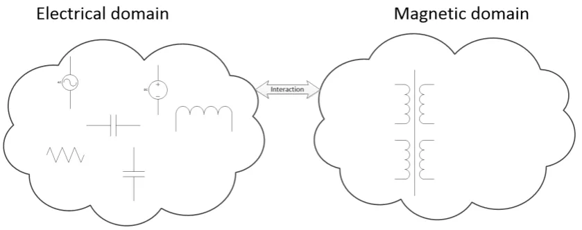
Furthermore, this work makes it straightforward to include the complex power transformer in electrical network analysis as the coupled inductors are mapped to an inductance matrix, which can be handled in electrical domain using the commonly available solvers such as EMTP/ATP or Spice (Fig. 1.). In the next section a method is described, where the transformer core and winding configuration are mapped to an inductance matrix. Section 3 shows a method to include the the transformer inductance matrix in nodal analysis and EMTP/ATP electric circuit solver. Section 4 shows two examples transformers and their surrounding circuits, where the method has been applied.

Figure 1, Magnetic circuit system interacting with electrical circuitry

2. Matrix representation of a complex inductor

Referring to Fig. 2, some topological concepts related to magnetic circuits are defined:

• Any magnetic circuit can be considered to consist of a set of interconnected limbs, which form a reluctance network.

• Fluxes in the limbs, that terminate to a node add up to zero (Kirchoff law electrical

(3)

• Magnetomotive force in any loop of limbs equals to the sum of limb reluctance times flux in the limb (Ohm law electrical analogy).

• There are windings in some, but not on all limbs.

Picture 2, Magnetic circuit topological definitions

Proposed method of modeling a coupled inductor is made in the following steps:

• Establish a winding matrix N, which links currents in the windings to magnetomotive

forces in the limbs.

• Establish a permeance matrix P, which maps currents in the limbs to fluxes in the limbs. Permeance matrix is calculated from the reluctance network using standard circuit analysis methods.

• Having established permeance matrix P and winding matrix N, the relationship

between currents in the windings and fluxes in the limbs is:

φ

=

PNI

.

• Multiplying limb fluxes by transpose of N and taking derivative1_{on time gives the}

voltages induced in the windings given the currents in them:

V

=

sN

T

PNI

.

• The matrix term

N

T

PN

is interpreted as a generalized inductance

L

_T , which is a complete representation of the coupled inductor using data from the winding and permeance matrices.

2.1 Winding matrix

Transformer windings carry currents and are represented by vector I. Let it's dimension be

n

_I

.

        

 

        

 

=

1

. .

4 3 2 1

n I

I I I I

I

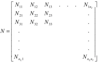
There is a mapping matrix N, which maps the currents in the windings to currents in the limbs. It's dimensions are nL×nI, where nL is the number of limbs.

(4)

                      = I L L I n n n n N N N N N N N N N N N N N 1 33 32 31 23 22 21 1 13 12 11 . . . . . . . . . . .

For example:

N

₃₁ means the number of windings current 1 has on limb 32_.

As illustrative example zig zag earthing transformer in Fig. 3 can be represented by the following N matrix:

          = A B A B B A N N N N N N N 0 0 0

Figure 3, Zig-zag winding

2.2 Describing the magnetic core with permeance matrix P

Core characteristics are in this analysis represented by a permeance matrix P. It maps magnetomotive forces in the limbs to fluxes in the limbs. It's dimensions are nL×nL so it is a square

matrix.                       = L L L L n n n n P P P P P P P P P P P P P 1 33 32 31 23 22 21 1 13 12 11 . . . . . . . . . . .

In order to derive permeance matrix of a transformer core, the transformer core is considered as a reluctance network. Once having the reluctance network, permeance matrix is calculated from the reluctance network using standard circuit analysis methods, taking into considering the magnetic-electric analogues. Consider, for example, a reluctance network of a three limb transformer as presented in Fig. 4.

2_{Note: the individual matrix elements Nij can be negative, if the winding is in reverse direction}

(5)

Figure 4, Reluctance network of single phase transformer with leakage flux path

The numbers in the boxes in reluctance network above refer to loops. The three limbs are numbered and the positive directions of the fluxes are marked. Then standard circuit analysis methods are applied to solve this circuit. R matrix is square containing the leakage (

R

₀) and limb (

L

R

)3_reluctances:













−

+

=

L L L L

R

2

0

Additionally the fluxes in the limbs are mapped to the fluxes in the loops. The transformer above has 3 limbs and 2 loops. This creates a conversions matrix Q of dimensions 3 X 2. The conversion matrix for the presented reluctance network is:













−

=

1

0

1

Q

In other words: multiplying with Q vector composed of magnetomotive forces in the limbs gives a vector of magnetomotive forces in the loops.

Applying these two matrices R and Q permeance matrix is calculated:

Q

R

Q

P

=

T −1

(1) As an illustration, the permeance matrix for the single phase transformer in Fig. 4 as above is:

                  + + + − + − + − + + + − + − + − + 2 0 0 2 0 0 0 2 0 0 2 0 0 0 0 0 0 2 2 2 1 2 2 2 1 2 1 2 1 2 2 L L L L L L L L L L L L L L L R R R R R R R R R R R R R R R R R R R R R R R R R R R R

2.3 Generalized transformer inductance matrix

Fluxes in the limbs can be calculated multiplying the magnetomotive forces in the limbs NI by permeance matrix P:

PNI

=

φ

₍₂₎

Multiplying limb fluxes by transpose of N and taking derivative on time gives the voltages induced in the windings given the currents in them. This means, that the generalized inductance

T

L

of the coupled inductor can be expressed in terms of the winding (N) and permeance (P)

matrices.

3_{Note a slightly different use for the term as compared to the topology definition above. Limb}

(6)

PNI

sN

V

=

T

PN

N

L

T

=

(3)

As an example, the complete inductance matrix single phase inductor in Fig. 4, is:

            + + + − + − + + 2 0 0 2 2 0 0 2 0 0 2 0 0 2 2 2 2 2 L L L P L L S P L L S P L L L P R R R R R N R R R R N N R R R R N N R R R R R N

In a limit, where R0 goes to infinity an intuitively clear form for L comes out, described below,

where L

P

R

N

2

and L

S

R

N

2

represent the primary and secondary self inductances and L

S P

R

N

is the mutual inductance.             − − L P L S P L S P L P R N R N N R N N R N 2 2 2 2 2 2

3. Integrating the generalized inductance to circuit solvers

The method presented above provides a straightforward and systematic way to derive inductance matrix for coupled inductors of any size and complexity. Naturally, the real value of the method becomes clear, when the number of limbs in the transformer exceeds three and where the reluctances are not symmetrical.

In any practical analysis the generalized inductance of coupled inductor system should be included in the analysis of the surrounding electrical circuit. Regarding this two practical cases can be considered: integrating coupled inductor in nodal analysis and incorporating the inductance matrix with numerical circuit solvers such as alternative transient analysis EMTP/ATP.

3.1 Integrating coupled inductor matrix to nodal analysis

3.1.1 Coupled inductor as voltage controlled current source vector

Typically larger electrical circuits and power networks are solved using nodal analysis [11]. List of nodes is constructed and the admittances between the nodes and the ground are included in the admittance matrix YN. Current sources are represented as a vector I denoting the currents arriving at

each individual node. Then the voltage in the nodes can be solved by solving the matrix equation:

I

V

Y

_N

=

(4)

The coupled inductor and it’s generalized inductance matrix can be integrated into the nodal system of equations by taking into consideration that it adds to the currents in similar way as the current sources. Effectively, any coupled inductor is a voltage controlled current source: voltage presented in windings manifests as currents in the windings as the inductance matrix dictates.

J

I

V

Y

_N

=

−

(5)

Thus, the inductance matrix L of the coupled inductor can be taken into consideration by considering the inductor as a current source J, driven by the scaled integral of the voltages in the coupled inductor’s windings. As the numbering of transformer windings differ from the numbering

of the nodes a conversion matrix mapping is required (

Λ

), which maps windings at coupled

inductors to the nodes in the nodal analysis. The transpose

Λ

Tmaps in the reverse direction. Considering, that node voltages are represented by vector V and the current source is J:

V

L

s

J

=

1

Λ

T −1

Λ

₍₆₎

(7)

V

L

s

I

V

Y

T

N

=

−

Λ

−1

Λ

1

(7)

Solving for node voltages V:

I

V

L

s

Y

V

T

1 1

1

₋ −













Λ

+

=

(8)

Thus, to incorporate complex coupled inductors to nodal electrical circuit analysis, the following steps will solve the complete electric-magnetic problem:

• Identify the inductance matrix (L) of the coupled inductor as presented above.

• Analyze the electrical circuit using the traditional nodal analysis method to come up with the admittance matrix (Y) of the electrical network.

• Find out the mapping between coupled inductor winding circuits and nodal voltages

Λ

.

• Calculate phasors or Laplace representations of the nodal voltages using (8).

With these steps the electric-magnetic problem can be solved systematically in a data-driven manner for any complexity for magnetic and electric networks.

3.1.2 Interpretation of coupled inductor as an additional admittance matrix

The previous chapter provided a result, where the coupled inductor introduces a voltage controlled current source vector to be added to the nodal currents. This can be brought one step

further for an additional insight. The matrix

L

V

s

Y

T

L

=

Λ

−1

Λ

1

can be considered also as an

admittance, as it gives the currents in the windings, given the voltages the voltages in them. Noting

the original source currents in nodal analysis as

Y

_N and that there are a number of coupled

inductors represented by their derived admittance matrices

Y

_L₁,

Y

_L₂…

Y

_LN then a modified nodal equation becomes:

I

V

Y

_N

+

_L

+

_L

+

_L

+

_LN

)

=

(

₁ ₂ ₃ (9)

This gives another interpretation for the method presented. For all coupled inductors, that are connected to electrical network, a corresponding admittance matrix can be created. These admittance matrices can simply be added to the admittance matrix of the electrical circuit and the entire circuit can then be solved using traditional solvers. This insight is usefull for analysis of larger electrical networks, which include multitude of transformers in different locations of the network.

3.2 Integrating to EMTP/ATP transient analysis

(8)

Figure 5, Principle for simulating the coupled inductor4

4. Examples

4.2 Example 1: Single phase transformer with leakage flux

Consider the transformer as presented in Fig. 6. It has primary and secondary windings in two separate limbs each having reluctance of RL and there is a path for the leakage flux via reluctance R0.

Figure 6, Reluctance model of transformer under study

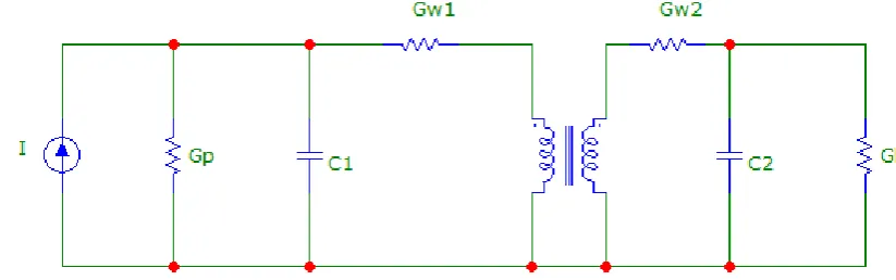
This transformer has winding resistances and capacitances and is driven by a Norton source and loaded by a resistive load. The surrounding electrical network is presented in Fig. 7. Gw1 and

represent Gw2s the primary and secondary winding conductances, while Gp include the combined

effect of source admittance and the core loss, C1 and C2 are the primary and secondary winding

capacitances respectively. GL is the load admittance and I is the current source.

Figure 7, Transformer and its electrical connections

4

The resistors are of very high value and are required by the EMTP/ATP solver for

numerical integration.

MODEL inductor

I

(9)

4.2 Nodal analysis

In chapter 1.4 inductance matrix of this magnetic circuit was derived. The nodal admittance matrix YN can be derived straightforwardly:

            + + − − − − + + = 2 2 2 2 2 1 1 1 1 1 0 0 0 0 0 0 0 0 sC G G G G G G G G sC G G Y L W W W W W W W W P N

The current source vector I is:

            = 0 0 0 V G I P

The matrix coupling the magnetic and electric parts is:

      = Λ 0 1 0 0 0 0 1 0

The magnetic addition

Y

_L to the nodal matrix can be calculated by (8) and it becomes:

                + + 0 0 0 0 0 0 0 0 0 0 0 0 2 0 0 0 2 0 P L S P S P P L sN R R N sN R N sN R sN R R

The complete admittance matrix

Y

_Ttaking into consideration both the magnetic and electric parts is:                 + + − − + + + + − − + + = 2 2 2 2 2 0 2 0 0 2 0 1 1 1 1 1 0 0 0 0 0 0 sC G G G G sN R R G N sN R N sN R sN R R G G G sC G G Y L W W W P L W S P S P P L W W W W P N

Inverting this matrix

Y

_Tand multiplying with current source vector I the nodal voltages come out. To demonstrate the function of the method, Fig. 8 below illustrates two situations, where the leakage reluctance is 50 times the reluctance of the limbs (blue) and 200 times the reluctance of the limbs (orange). It shows the known phenomenon, that the leakage reluctance makes the output voltage drop at high loads.

Figure 8, Output voltage of the transformer under study at different resistive loads

(10)

Figure 9, Output voltage transient of the transformer under analysis

4.3 EMTP/ATP analysis

The transformer under study was modeled with ATPDRAW using method described above. The inverse of inductance matrix was calculated as:













.

1005

.

100

.

100

05

.

10

The simulated network is as in Fig. 10.

Fig. 10, Network to simulate the transformer under study

The transient produced by the electromagnetic solver is described in Figure 11.

Fig. 11, ATP generated transient for transformer under study

Referring to Fig. 9 in the previous chapter it can be seen, that the transients are equal. Thus, this serves as a validation of the method in a non-trivial case.

0.005 0.010 0.015 0.020Time

0.02 0.04 0.06 0.08 0.10 Relative voltage

I

MODEL

lm

U V

(file single_phase_trafo_matrix_study_v1.pl4; x-var t) v:XX0002-

0 4 8 12 16 *10-3 20

(11)

4.2 Example 2: three phase three limb reactor with yoke reluctances and leakage flux

Another practical non-trivial example analyzed is: three phase three limb reactor with yoke reluctances and leakage flux paths. A target is to use the modeling presented to study, how the asymmetries created by yoke and leakage reluctances impact the symmetry of currents. The relevance of this is due to the fact, that transformer analysis literature there are no systematic methods to deal with transformer cores with significant asymmetries. Target is to see, how that impacts the asymmetry of the core impact the output voltages at different loads. The analyzed reactor is presented in Fig.13 and the surrounding electrical network is in Fig. 12.

Figure 12, Reactor and the surrounding electrical circuit

Figure 13, Three phase three limb reactor with yoke reluctances and leakage flux

4.3.1 Matrices

Considering the reactor in pictures 12 and 13, the descriptive matrices N, R and Q as well as the nodal matrix YN are:

(12)













P P P

N

0

R:                 + − − + + − − + − − + + − − + L Y L L L L Y L L L R R R R R R R R R R R R R R R R R R R R 0 0 0 0 0 0 0 0 0 0 0 0 0 0 0 0 0 0 0 0 0 0 Q:













−

1

0

1

0

1

0

1

0

1

From these matrices the inductance L matrix is calculated. When the yoke reluctances are zero and leakage reluctances go to infinity the inductance matrix becomes:













−

2

1

2

1

2

3

2 L P

R

N

The admittance matrix YN of the surrounding electrical network is:













−

+

w w w w w w w w w W

G

0

3

0

For numerical calculation the following parameters are assumed:

• NP=1000

• NP=100

• RL=5000 1/H • R0= 200 RL • RY= RL • GW=0.1 S

These parameter values correspond to a practical three phase reactor with 25 cm2_{cross sectional}

area for the magnetic core. Yoke and leakage reluctance evaluated based on finite element analysis of the said reactor.

(13)













0999548

.

0

0999998

.

0

10044

.

0

Currents in symmetrical components:













−

0999

.

0

000052

.

0

10

*

034

.

1

17

The negative sequence current is only about 0.5% of the positive sequence current and there is practically no zero sequence current. Thus, for a practical reactor, the approximation, where yoke reluctances are zero is quite applicable, contrary to intuition.

5. Conclusions

A data-driven and matrix oriented method was presented in which complex coupled inductors of any complexity can be analyzed with the surrounding electrical network in a systematic way. The transformer structure is presented in four matrices N,R,Q and P, that are easily extracted from the physical measures and material specifications of the transformer. Result is a generalized inductor matrix, which in turn can be transformed to an admittance matrix, which can be integrated into traditional nodal circuit analysis and electrical transient solvers such as EMTP/ATP.

Using the methods presented a number of complex transformer structures has been analyzed and validated and the method can be used for modeling linear coupled inductors of any complexity in networks of any size.

Conflicts of Interest: The authors declare no conflict of interest.

References

1. S. Kulkarni, S. Khaparde,”Transformer Engineering”, CRC Press, 2012, Second Edition, ISBN:

978-1-4398-5377-1.

2. R. Del Vecchio, B. Poulin, P. Feghali, D. Shah, R. Ahuja, “Transformer Design Principles”, CRC Press, 2010, Second Edition, ISBN: 978-1-4398-0582-4.

3. Xusheng, “A Three-Phase Three Winding Core-type transformer Model for Low-Frequency

Transient Studies”, IEEE Transactions on Power Delivery, Vol. 11, No. 3, July 1997.

4. E: teNyienhuis, G. Mechler, R: Girgis, “Flux Distribution and Core Loss Calculation for Single Phase and Five Limb Three Phase Transformer Core Designs”, IEEE Transactions on Power Delivery, Vol. 15, No. 1, January 2000.

5. Dzafiq, R. Jabr, H. Neisius, ”Transformer Modeling for Three-Phase Distribution Network

Analysis”, IEEE Transactions on Power Systems, Vol 30, No 5, September 2015.

6. M. Irving, A. Al-Othman, “Admittance Matrix Models of Three-Phase Transformers with

Various Neutral Grounding Configurations”, IEEE Transactions on Power Systems, Vol 18, No 3, August 2003.

7. X. Chen, “A Three-Phase Multi-Legged Transformer Model in ATP Using the Directly Formed

Inverse Inductance Matrix”, IEEE Transactions on Power Delivery, Vol 11, No. 3, July 1995.

8. F. Corcoles, L. Sainz, J. Pedra, J. Sancez-Navarro, M. Salichs, “Three-phase transformer

(14)

9. J. Elovaara, L. Haarla, “Sähköverkot I”, Gaudeamus Helsinki University Press, Tallinna, 2011, ISBN: 978-951-672-360-3.

10. Baktash, A. Vahedi, “Modeling of tape wound cores using reluctance networks for distribution transformers”, International Power System Conference 27-29 October 2014, Tehran.

11. S. Sarma, J. Glover, T. Overbye, “Power System Analysis and Design”, Cengage Learning,

2012,Fifth Edition, ISBN-10: 1111425779.

12. Micro_Cap 11, Electronic Circuit Analysis Program User’s Guide, Spectrum Software, Version 11, 2014 Spectrum Software.

13. ATPDRAW, version 5.6, for Windows 9x/NT/2000/XP/Vista, User’s manual, 2009.