Comparing Supervised Machine Learning Strategies
and linguistic Features to Search for Very Negative
Opinions
Sattam Almatarneh1,†,* and Pablo Gamallo1
1 Centro Singular de Investigación en Tecnoloxías da Información (CITIUS), Universidad de Santiago de
Compostela, Rua de Jenaro de la Fuente Domínguez, Santiago de Compostela 15782, Spain;
* Correspondence: [email protected]; Tel.: +34631648949
Academic Editor: name
Version November 19, 2018 submitted to Preprints
Abstract:In this paper, we examine the performance of several classifiers in the process of searching 1
for very negative opinions. More precisely, we do an empirical study that analyzes the influence 2
of three types of linguistic features (n-grams, word embeddings, and polarity lexicons) and their 3
combinations when they are used to feed different supervised machine learning classifiers: Support 4
Vector Machine (SVM), Naive Bayes (NB), and Decision Tree (DT). 5
Keywords: Sentiment Analysis; Opinion Mining; linguistic features; Classification; Very negative 6
Opinions 7
1. Introduction 8
The information revolution is the most prominent feature of this century. The world has become 9
a small village with the proliferation of social networking sites where anyone around the planet can 10
sell, buy or express their opinions. The vast amount of information on the Internet has become a 11
source of interest for studies, as it offers an excellent opportunity to extract information and organize it 12
according to the particular needs. 13
After the massive explosion in the use of the Internet and social media in various aspects of life, 14
social media has come to play a significant role in guiding people’s tendencies in social, political, 15
religious and economic domains, through the opinions expressed by individuals. 16
Sentiment Analysis also called Opinion Mining is defined as the field of study that analyzes 17
people’s opinions, sentiments, evaluations, attitudes, and emotions from written language. It is one of 18
the most active research areas in Natural Language Processing (NLP) and is also widely studied in 19
data mining, Web mining, and text mining [1]. 20
Sentiment analysis typically works at four different levels of granularity, namely document level, 21
sentence level, aspect level, and concept level. Most early studies in Sentiment Analysis [2,3] put 22
their focus at document level and relied on datasets such as movie and products reviews. After the 23
widespread of the Internet and e-commerce boom, different types of datasets have been collected from 24
websites about customer opinions. The review document often expresses opinions on a single product 25
or service and was written by a single reviewer. 26
According to Panget al.[4], 73% and 87% among readers of online reviews such as (restaurants, 27
hotels, travel agencies or doctors), state that reviews had a significant influence on their purchase. 28
The fundamental task in Opinion Mining is polarity classification [5–7], which occurs when a 29
piece of text stating an opinion is classified into a predefined set of polarity categories (e.g., positive, 30
neutral, negative). Reviews such as "thumbs up" versus "thumbs down", or "like" versus "dislike" are 31
examples of two-class polarity classification. An unusual way of performing sentiment analysis is to 32
detect and classify opinions that represent the most negative opinions about a topic, an object or an 33
individual. We call themextreme opinions. 34
The most negative opinion is the worst view, judgment, or appraisal formed in one’s mind about 35
a particular matter. People always want to know the worst aspects of goods, services, places, etc. so 36
that they can avoid them or fix them. The very negative views have a strong impact on product sales 37
since they influence customer decisions before buying. Previous studies analyzed this relationship, 38
such as the experiments reported in [8], which found that as the high proportion of negative online 39
consumer reviews increased, the consumer’s negative attitudes also increased. Similar effects have 40
been observed in consumer reviews: one-star reviews significantly hurt book sales on Amazon.com 41
[9]. The impact of 1-star reviews, which represent the most negative views, is greater than the impact 42
of 5-star reviews in this particular market sector. 43
The main objective of this article is to examine the effectiveness and limitations of different 44
linguistic features and supervised sentiment classifiers to identify the most negative opinions in 45
four domains reviews. It is an expanded version of a conference paper presented at KESW 2017 46
[10]. Our main contribution is to report an extensive set of experiments aimed to evaluate the 47
relative effectiveness of different linguistic features and supervised sentiment classifiers for a binary 48
classification task, namely to search for very negativevs.not very negative opinions. 49
The rest of the paper is organized as follows. In the following section (2), we discuss the related 50
work. Then, Section3describes the method. Experiments are introduced in Section4, where we also 51
describe the evaluation and discuss the results. We draw the conclusions and future work in Section5. 52
2. Related Work 53
There are two main approaches to find the sentiment polarity at a document level. First, machine 54
learning techniques based on training corpora annotated with polarity information and, second, 55
strategies based on polarity lexicons. 56
In machine learning, there are two main methods, unsupervised and supervised learning, even 57
though only the later strategy is used by most existing techniques for document-level sentiment 58
classification. Supervised learning approaches use labeled training documents based on automatic text 59
classification. A labeled training set with a pre-defined categories is required. A classification model is 60
built to predict the document class on the basis of pre-defined categories. The success of supervised 61
learning mainly depends on the choice and extraction of the proper set of features used to identify 62
sentiments. There are many types of classifiers for sentiment classification using supervised learning 63
algorithms: 64
• Probabilistic classifiers like Naive Bayes, Bayesian network, and maximum entropy. 65
• Decision tree classifiers, whcih build a hierarchical tree-like structure with true/false queries 66
based on categorization of training documents. 67
• Linear classifiers, which separate input vectors into classes using linear (hyperplane) decision 68
boundaries. The most popular linear classifiers are Support Vector Machine (SVM) and neural 69
networks(NN). 70
One of the pioneer research on document-level sentiment analysis was conducted by Panget al.
71
[3] using Naive Bayes (NB), Maximum Entropy (ME), and SVM for binary sentiment classification of 72
movie reviews. They also tested different features, to find out that SVM with unigrams yielded the 73
highest accuracy. 74
SVM is one of the most popular supervised classification methods. It has a robust theoretical 75
base, is likely the most precise method in text classification [11] and is also successful in sentiment 76
classification [12–14]. It generally outperforms Naive Bayes and finds the optimal hyperplane to divide 77
classes [15]. Moraeset al.[16] compared SVM and NB with Artificial Neural Network (NN) approaches 78
for sentiment classification. Experiments were performed on the both balanced and unbalanced 79
dataset. For this purpose, four datasets were chosen, namely movies review dataset [17] and three 80
different products review (GPS, Books, and Cameras). For unbalanced dataset, the performances of 81
of three techniques, namely Naive Bayes, Decision Tree, and Nearest Neighbour, in order to classify 83
Urdu and English opinions in a blog. Their results show that Naive Bayes has better performance 84
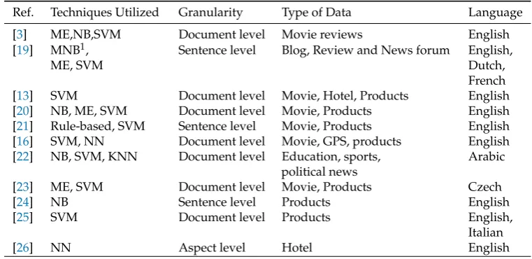
than the other two. Table1summarizes the main components of some published studies: techniques 85
utilized, the granularity of the analysis (sentence-level or document-level, etc.), type of data, source of 86
data, and language.
Table 1.Main components of some supervised learning sentiment classification published studies.
Ref. Techniques Utilized Granularity Type of Data Language
[3] ME,NB,SVM Document level Movie reviews English
[19] MNB1, ME, SVM
Sentence level Blog, Review and News forum English, Dutch, French
[13] SVM Document level Movie, Hotel, Products English
[20] NB, ME, SVM Document level Movie, Products English
[21] Rule-based, SVM Sentence level Movie, Products English
[16] SVM, NN Document level Movie, GPS, products English
[22] NB, SVM, KNN Document level Education, sports,
political news
Arabic
[23] ME, SVM Document level Movie, Products Czech
[24] NB Sentence level Products English
[25] SVM Document level Products English,
Italian
[26] NN Aspect level Hotel English
87
The quality of the selected features is a key factor in increasing the efficiency of the classifier for 88
determining the target. Some typical features are n-grams, word embedding, and sentiment words. 89
These features have been employed by different researchers. 90
The influence of this type of content features has been analyzed by several opinion mining studies 91
[3,27,28]. 92
Tripathyet al.[29] proposed an approach to find the polarity of reviews by converting text into 93
numeric matrices using countvectorizer and TF-IDF, and then using it as input in machine learning 94
algorithms for classification. Martín-Valdiviaet al. [30] combined supervised and unsupervised 95
approaches to get a meta-classifier. Term Frequency-Inverse Document Frequency (TF-IDF), Term 96
Frequency (TF), Term Occurrence (TO), and Binary Occurrence (BO) were considered as feature 97
representation schemes. SVM outperformed NB for both corpora. TF-IDF was reported as the better 98
representation scheme. SVM using TF-IDF without stopword and stemmer yielded the best precision. 99
Paltoglou and Thelwall [31] examined different unigram weighting schemes and found that some 100
variants of TF-IDF are well suited for Sentiment Analysis. 101
Sentiment words also called opinion words are considered the primary building block in sentiment 102
analysis as they represent an essential resource for most sentiment analysis algorithms, and the first 103
indicator to express positive or negative opinions. There are, at least, two ways of building sentiment 104
lexicons: hand-craft elaboration [32–35], and automatic construction on the basis of external resources. 105
Two different automatic strategies may be identified according to the nature of these resources: 106
thesaurus and corpora. 107
[36] described the creation of two corpus-based lexicons. First, a general lexicon using 108
SentiwordNet and the Subjectivity Lexicon. Second, a domain-specific lexicon using a corpus of 109
drug reviews depending on statistical information. [37] built a lexicon containing a combination of 110
sentiment polarity (positive, negative) with one of eight possible emotion classes (anger, anticipation, 111
disgust, fear, joy, sadness, surprise, trust) for each word. 112
As far as we know, except our previous works [10,38] no other previous work has been focused 113
on detecting very negative opinions. Our proposal, therefore, may be considered to be the first step in 114
3. Method 116
In this section, we will describe the most important linguistic features and supervised sentiment 117
classifiers that we will use in our experiments. 118
We have focused on the selection of influential linguistic features taking into account the 119
importance of the quality of the selection of features as a key factor in increasing the efficiency 120
of the classifier in determining the target. The main linguistic features we will use and analyze are the 121
following: N-grams, word embeddings, and sentiment lexicons. 122
3.1. N-grams Features
123
We deal with n-grams based on the occurrence of unigrams and bigrams of words in the document. 124
Unigrams (1g) and bigrams (2g) are valuable to detect specific domain-dependent (opinionated) 125
expressions. 126
We assign a weight to all terms by using two different representations: TF-IDF and 127
CountVectorizer. 128
TF-IDF is computed in Equation1.
t f/id ft,d= (1+log(t ft,d))×log(
N d ft
). (1)
wheret ft,dis the term frequency of the termtin the documentd,Nis the number of documents in the 129
collection and,d ftis the number of documents in the collection containingt. 130
CountVectorizer transforms the document to token count matrix. First, it tokenizes the document 131
and according to a number of occurrences of each token, a sparse matrix is created. In order to create 132
the Matrix, all stopwords are removed from the document collection. Then, the vocabulary is cleaned 133
up by removing those terms appearing in less than 4 documents to filter out those terms that are too 134
infrequent. 135
To convert the reviews to a matrix of TF-IDF features and to a matrix of token occurrences, we 136
usedsklearnfeature extraction python library.2 3 137
3.2. Word Embedding
138
Many deep learning models in NLP need word embedding results as input features. Word 139
embeddings is a technique for language modeling and feature learning, which converts words 140
in a vocabulary into vectors of continuous real numbers representing their semantic distribution. 141
The technique commonly involves embedding from a high-dimensional sparse vector space into a 142
lower-dimensional dense vector space. Each dimension of the embedding vector represents a latent 143
feature of a word. The vectors may encode linguistic regularities and patterns of the word contexts. 144
The acquisition of word embeddings can be done using neural networks. 145
We used thedoc2vecalgorithm introduced in Le and Mikolov [39] to represent the reviews. This 146
neural-based representation has been shown to be efficient when dealing with high-dimensional and 147
sparse data [39,40]. Doc2vec learns features from the corpus in an unsupervised manner and provides 148
a fixed-length feature vector as output. Then, the output is fed into a machine-learning classifier. We 149
used a freely available implementation of the doc2vec algorithm included in gensim,4which is a free 150
Python library. The implementation of the doc2vec algorithm requires the number of features to be 151
returned (length of the vector). So, we performed a grid search over the fixed vector length 100 [41–43]. 152
2 http://scikit-learn.org/stable/modules/generated/sklearn.feature_extraction.text.CountVectorizer.html
3 http://scikit-learn.org/stable/modules/generated/sklearn.feature_extraction.text.TfidfVectorizer.html#sklearn.feature_ extraction.text.TfidfVectorizer
3.3. Sentiment Lexicons
153
Sentiment words, also called opinion words, are considered the primary building block in 154
sentiment analysis as it is an essential resource for most sentiment analysis algorithms, and the 155
first indicator to express positive or negative opinions. Also, many textual features may be used 156
as pieces of evidence to detect very negative views. In this study, we have extracted some of them 157
to examine to what extent they influence the identification of extreme views (very negative ones). 158
Uppercase characters may indicate that the writer is very upset, so we counted the number of words 159
written in uppercase letters. Also, intensifier words could be a reliable indicator of the existence of 160
very negative views. So, we considered words such asmostly, hardly, almost, fairly, really, completely,
161
definitely, absolutely, highly, awfully, extremely, amazingly, fully, and so on. 162
Furthermore, we took into account negation words such asno, not, none, nobody, nothing, neither,
163
nowhere, never, etc. In addition, we also considered elongated words and repeated punctuation such as 164
sooooo, baaaaad, woooow, gooood, ???, !!!!, etc.. These textual features have been shown to be effective in 165
many studies related to polarity classification such as Taboadaet al.[32], Kennedy and Inkpen [44]. In 166
our previous studies [45,46], we described a strategy to build sentiment lexicons from corpora. In the 167
current study, we will use our lexicon, called VERY-NEG5which contains a list of very negative words 168
(VN) and a list of words that are not considered to be very negative (NVN). VERY-NEG lexicon was 169
built from the text corpora described in Potts [47]. The corpora6consist of online reviews collected 170
from IMDB, Goodreads, OpenTable and Amazon/Tripadvisor. Each of the reviews in this collection 171
has an associated star rating: one star (very negative) to ten stars (very positive) in IMDB, and one star 172
(very negative) to five stars (very positive) in the other online reviews. 173
Reviews were tagged using the Stanford Log-Linear Part-Of-Speech Tagger. Then, tags were 174
broken down into WordNet PoS Tags:a(adjective),n(noun),v(verb),r(adverb). Words whose tags 175
were not part of those categories were filtered out. The list of selected words was then stemmed. 176
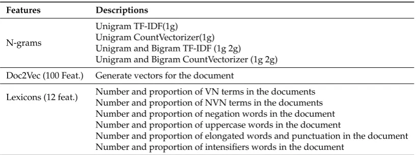
Table2summarizes all the features introduced above with a brief description for each one. 177
Table 2.Description of all linguistic features.
Features Descriptions
N-grams
Unigram TF-IDF(1g)
Unigram CountVectorizer(1g) Unigram and Bigram TF-IDF (1g 2g)
Unigram and Bigram CountVectorizer (1g 2g)
Doc2Vec (100 Feat.) Generate vectors for the document
Lexicons (12 feat.) Number and proportion of VN terms in the documents Number and proportion of NVN terms in the documents Number and proportion of negation words in the document Number and proportion of uppercase words in the document
Number and proportion of elongated words and punctuation in the document Number and proportion of intensifiers words in the document
4. Experiments 178
4.1. Multi-Domain Sentiment Dataset
179
This dataset7was used in Blitzeret al.[48]. It contains product reviews taken from Amazon.com 180
for 4 types of products (domains): Kitchen, Books, DVDs, and Electronics. The star ratings of the 181
5 https://github.com/almatarneh/LEXICONS
6 http://www.stanford.edu/~cgpotts/data/wordnetscales/
reviews are from 1 to 5 stars. In our experiments, we adopted the scale with five categories. In this 182
case, the borderline separating the VN values from the rest was set to 1, which stands for the very 183
negative reviews. The documents in the other four categories were put in the not very negative (NVN) 184
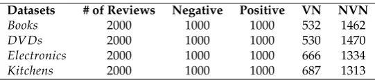
class. Table3shows the number of reviews in each class for each task. 185
Table 3.Size of the four test datasets and the total number of reviews in each class negativevs.positive and (VNvs.NVN )
Datasets # of Reviews Negative Positive VN NVN
Books 2000 1000 1000 532 1462
DVDs 2000 1000 1000 530 1470
Electronics 2000 1000 1000 666 1334
Kitchens 2000 1000 1000 687 1313
4.2. Training and Test
186
Since we are facing a text classification problem, any existing supervised learning method can be 187
applied. Support Vector Machines (SVM), Naive Bayes (NB), and Decision Tree (DT) has been shown 188
to be highly effective at traditional text categorization [3]. We decided to utilizescikit8, which is an 189
open source machine learning library for Python programming language [49]. We chose SVM, NB and 190
DT as our classifiers for all experiments, hence, in this study we will compare, summarize and discuss 191
the behaviour of these learning models with the linguistic features introduced above. Supervised 192
classification requires two samples of documents: training and testing. The training sample will be 193
used to learn various characteristics of the documents and the testing sample was used to predict and 194
next verify the efficiency of our classifier in the prediction. The data set was randomly partitioned into 195
training (75 %) and test (25 %). 196
In our analysis, we employed 5_fold cross_validation and the effort was put on optimizing F1 197
which is computed with respect to very negative (VN) (which is the target class): 198
F1=2∗ P∗R
P+R (2)
wherePandRare defined as follows:
P= TP
TP+FP (3)
R= TP
TP+FN (4)
Where TP stands for true positive, FP is false positive, and FN is false negative. 199
4.3. Results
200
Tables4,5,6and7Polarity classification results by SVM, NB, DT classifiers for all dataset with all 201
linguistic features alone and combined together, in terms of Precision (P), Recall (R) and F1 scores for 202
very negativeclass (VN). 203
Table 4.Polarity classification results by SVM, NB, DT classifiers for Book dataset with all linguistic features alone and combined together, in terms of Precision (P), Recall (R) and F1 scores forvery negative
class (VN). The best F1 is highlighted (in bold).
BOOk Features SVM Naive Bayes Decision Tree
P R F1 P R F1 P R F1
1gTF-IDF 0.62 0.34 0.44 0.33 0.18 0.23 0.46 0.36 0.40
1gCountVector 0.55 0.51 0.53 0.34 0.20 0.25 0.41 0.38 0.39
1g2gTF-IDF 0.68 0.34 0.45 0.43 0.14 0.21 0.43 0.36 0.39
1g2gCountVector 0.57 0.49 0.53 0.45 0.15 0.23 0.43 0.41 0.42
Doc2Vec 0.57 0.32 0.41 0.46 0.62 0.53 0.40 0.40 0.40
Lexicon 0.81 0.18 0.29 0.51 0.27 0.35 0.42 0.38 0.40
Doc2Vec+Lexicon 0.64 0.44 0.52 0.61 0.45 0.52 0.42 0.42 0.42
1gTF-IDF + Doc2Vec 0.63 0.49 0.55 0.34 0.18 0.23 0.45 0.42 0.43
1gTF-IDF +Lexicon 0.67 0.41 0.51 0.35 0.18 0.24 0.47 0.40 0.43
1gTF-IDF +Doc2Vec+Lexicon 0.64 0.51 0.57 0.35 0.18 0.24 0.47 0.43 0.45
1gCountVector +Doc2Vec 0.56 0.52 0.54 0.34 0.20 0.25 0.43 0.40 0.42
1gCountVector+Lexicon 0.59 0.51 0.55 0.34 0.20 0.25 0.53 0.42 0.47
1gCountVector +Doc2Vec+Lexicon 0.59 0.51 0.55 0.34 0.20 0.25 0.47 0.43 0.45
1g2gTF-IDF + Doc2Vec 0.63 0.49 0.55 0.44 0.14 0.21 0.44 0.39 0.41
1g2gTF-IDF +Lexicon 0.69 0.38 0.49 0.47 0.14 0.21 0.48 0.43 0.46
1g2gTF-IDF +Doc2Vec+Lexicon 0.64 0.51 0.56 0.47 0.14 0.21 0.48 0.40 0.44
1g2gCountVector+Doc2Vec 0.58 0.51 0.54 0.45 0.15 0.23 0.45 0.47 0.46
1g2gCountVector+Lexicon 0.58 0.49 0.53 0.45 0.15 0.23 0.46 0.43 0.45
1g2gCountVector+Doc2Vec + Lexicon 0.60 0.54 0.57 0.45 0.15 0.23 0.48 0.43 0.45
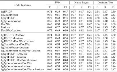
Table 5.Polarity classification results by SVM, NB, DT classifiers for DVD dataset with all linguistic features alone and combined together, in terms of Precision (P), Recall (R) and F1 scores forvery negative
class (VN). The best F1 is highlighted (in bold).
DVD Features SVM Naive Bayes Decision Tree
P R F1 P R F1 P R F1
1gTF-IDF 0.74 0.35 0.47 0.37 0.17 0.24 0.54 0.47 0.50
1gCountVector 0.56 0.51 0.53 0.37 0.17 0.24 0.47 0.40 0.43
1g2gTF-IDF 0.70 0.33 0.45 0.50 0.11 0.18 0.48 0.46 0.47
1g2gCountVector 0.56 0.49 0.52 0.50 0.11 0.18 0.48 0.40 0.44
Doc2Vec 0.67 0.30 0.42 0.33 0.81 0.47 0.36 0.41 0.38
Lexicon 0.69 0.27 0.38 0.49 0.57 0.53 0.46 0.45 0.45
Doc2Vec+Lexicon 0.72 0.49 0.58 0.34 0.82 0.48 0.47 0.47 0.47
1gTF-IDF + Doc2Vec 0.74 0.48 0.58 0.37 0.17 0.24 0.56 0.45 0.50
1gTF-IDF +Lexicon 0.72 0.43 0.54 0.37 0.17 0.23 0.53 0.50 0.51
1gTF-IDF +Doc2Vec+Lexicon 0.69 0.52 0.59 0.37 0.17 0.23 0.48 0.45 0.46
1gCountVector +Doc2Vec 0.59 0.55 0.57 0.37 0.17 0.24 0.48 0.48 0.48
1gCountVector+Lexicon 0.59 0.53 0.56 0.37 0.17 0.24 0.46 0.40 0.43
1gCountVector +Doc2Vec+Lexicon 0.62 0.57 0.59 0.37 0.17 0.24 0.51 0.47 0.49
1g2gTF-IDF + Doc2Vec 0.72 0.50 0.59 0.50 0.11 0.18 0.53 0.44 0.48
1g2gTF-IDF +Lexicon 0.73 0.45 0.56 0.47 0.10 0.16 0.49 0.46 0.47
1g2gTF-IDF +Doc2Vec+Lexicon 0.71 0.52 0.60 0.47 0.10 0.16 0.51 0.42 0.46
1g2gCountVector+Doc2Vec 0.61 0.57 0.59 0.50 0.11 0.18 0.44 0.42 0.43
1g2gCountVector+Lexicon 0.62 0.55 0.58 0.50 0.11 0.18 0.51 0.42 0.46
Table 6.Polarity classification results by SVM, NB, DT classifiers for Electronic dataset with all linguistic features alone and combined together, in terms of Precision (P), Recall (R) and F1 scores forvery negative
class (VN). The best F1 is highlighted (in bold).
Electronic Features SVM Naive Bayes Decision Tree
P R F1 P R F1 P R F1
1gTF-IDF 0.69 0.57 0.63 0.49 0.41 0.45 0.58 0.58 0.58
1gCountVector 0.61 0.60 0.61 0.50 0.43 0.46 0.59 0.55 0.57
1g2gTF-IDF 0.70 0.56 0.62 0.58 0.37 0.45 0.55 0.51 0.53
1g2gCountVector 0.62 0.57 0.59 0.59 0.40 0.48 0.55 0.51 0.53
Doc2Vec 0.72 0.61 0.66 0.55 0.35 0.43 0.48 0.55 0.51
Lexicon 0.69 0.42 0.52 0.58 0.53 0.55 0.50 0.50 0.50
Doc2Vec + Lexicon 0.71 0.66 0.68 0.56 0.35 0.43 0.47 0.50 0.49
1gTF-IDF +Doc2Vec 0.68 0.67 0.68 0.50 0.41 0.45 0.53 0.50 0.52
1gTF-IDF +Lexicon 0.68 0.60 0.64 0.51 0.39 0.45 0.57 0.54 0.55
1gTF-IDF +Doc2Vec + Lexicon 0.73 0.66 0.69 0.51 0.39 0.45 0.59 0.51 0.55
1gCountVector +Doc2Vec 0.64 0.62 0.63 0.50 0.43 0.46 0.55 0.51 0.53
1gCountVector + Lexicon 0.63 0.61 0.62 0.50 0.43 0.46 0.57 0.47 0.52
1gCountVector +Doc2Vec + Lexicon 0.66 0.62 0.64 0.50 0.43 0.46 0.59 0.51 0.55
1g2gTF-IDF + Doc2Vec 0.76 0.61 0.68 0.58 0.37 0.45 0.53 0.52 0.52
1g2gTF-IDF + Lexicon 0.70 0.61 0.65 0.58 0.37 0.45 0.60 0.59 0.59
1g2gTF-IDF + Doc2Vec + Lexicon 0.69 0.69 0.69 0.58 0.37 0.45 0.67 0.59 0.63
1g2gCountVector + Doc2Vec 0.66 0.58 0.62 0.59 0.40 0.48 0.51 0.46 0.49
1g2gCountVector + Lexicon 0.65 0.59 0.62 0.59 0.40 0.48 0.54 0.49 0.51
1g2gCountVector + Doc2Vec + Lexicon 0.64 0.63 0.64 0.59 0.40 0.48 0.64 0.50 0.56
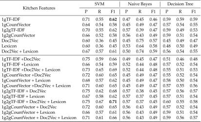
Table 7.Polarity classification results by SVM, NB, DT classifiers for Kitchen dataset with all linguistic features alone and combined together, in terms of Precision (P), Recall (R) and F1 scores forvery negative
class (VN). The best F1 is highlighted (in bold).
Kitchen Features SVM Naive Bayes Decision Tree
P R F1 P R F1 P R F1
1gTF-IDF 0.71 0.55 0.62 0.47 0.45 0.46 0.59 0.59 0.59
1gCountVector 0.64 0.54 0.58 0.45 0.49 0.47 0.57 0.54 0.55
1g2gTF-IDF 0.70 0.55 0.62 0.57 0.39 0.47 0.59 0.49 0.53
1g2gCountVector 0.66 0.52 0.58 0.56 0.43 0.49 0.59 0.51 0.54
Doc2Vec 0.60 0.36 0.45 0.45 0.75 0.57 0.45 0.49 0.47
Lexicon 0.60 0.36 0.45 0.53 0.64 0.58 0.48 0.50 0.49
Doc2Vec + Lexicon 0.67 0.57 0.61 0.50 0.74 0.59 0.56 0.54 0.55
1gTF-IDF +Doc2Vec 0.75 0.59 0.66 0.49 0.45 0.47 0.51 0.46 0.48
1gTF-IDF +Lexicon 0.66 0.54 0.59 0.52 0.44 0.48 0.57 0.52 0.54
1gTF-IDF +Doc2Vec + Lexicon 0.73 0.65 0.69 0.52 0.44 0.48 0.55 0.51 0.53
1gCountVector +Doc2Vec 0.72 0.60 0.65 0.45 0.49 0.47 0.55 0.52 0.54
1gCountVector + Lexicon 0.68 0.57 0.62 0.45 0.49 0.47 0.58 0.50 0.54
1gCountVector +Doc2Vec + Lexicon 0.71 0.60 0.65 0.45 0.49 0.47 0.57 0.55 0.56
1g2gTF-IDF + Doc2Vec 0.75 0.62 0.68 0.57 0.38 0.45 0.57 0.56 0.57
1g2gTF-IDF + Lexicon 0.67 0.58 0.62 0.57 0.37 0.45 0.57 0.51 0.54
1g2gTF-IDF + Doc2Vec + Lexicon 0.75 0.67 0.71 0.57 0.37 0.45 0.60 0.55 0.58
1g2gCountVector + Doc2Vec 0.72 0.60 0.65 0.56 0.43 0.49 0.57 0.52 0.54
1g2gCountVector + Lexicon 0.66 0.57 0.61 0.56 0.43 0.49 0.59 0.51 0.54
1g2gCountVector + Doc2Vec + Lexicon 0.71 0.61 0.66 0.56 0.43 0.49 0.59 0.56 0.57
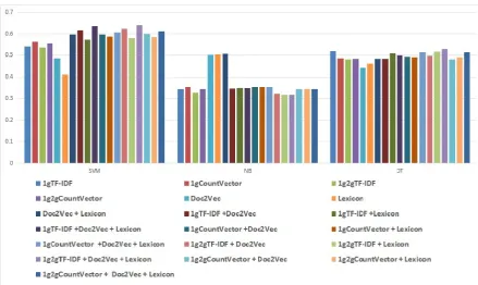
The results, which are quite low due to the difficulty of the task, show that SVM is by far the 204
Figure 1.Comparison between the polarity classification results by all classifiers for all collections with all features alone and after combined together, by computing the average of all F1 forvery negativeclass (VN).
tests. Figure1shows how SVM outperforms the other classifiers with all features and combinations of 206
features by computing the average of all F1 values across the four datasets. 207
The performance of NB differs greatly depending on the number of features used in classification. 208
NB works better with a small number of features, more precisely the best scores are achieved when it 209
only uses either Lexicon or Doc2Vec. It is worth noting that the combination of heterogeneous features 210
hurts the performance of this type of classifier. 211
The DT classifier has a similar behavior to SVM in terms of stability, but its performance tends to 212
be much lower than that of SVM, as can be seen in Figure1. 213
Concerning the linguistic features, the best performance of SVM (and thus of all classifiers) is 214
reached when combining TF-IDF, whether 1g or 2g, with Lexicon and Doc2Vec, as shown in Figure1. 215
So, the combination of all feature types (n-grams, embeddings and sentiment lexicon) gives rise to the 216
best results in our experiments. These results must be evaluated taking into account the enormous 217
difficulty of overcoming basic features such as n-grams, which are considered as a strong baseline in 218
tasks related to document-based classification. 219
Moreover, it should also be noted that the combination of just the lexicon and Doc2Vec 220
(Doc2Vec+Lexicon) works very well with SVM and DT. This specific combination clearly outperforms 221
the results obtained by just using either Lexicon or Doc2Vec alone, and even tends to perform better 222
than using just n-grams, which is considered a very strong baseline in this type of classification task. 223
5. Conclusions 224
In this article, we have studied different linguistic features for a particular task in Sentiment 225
Analysis. More precisely, we examined the performance of these features within supervised learning 226
methods (using SVM, NB, DT), to identify the most negative documents on four domains review 227
datasets. 228
The experiments reported in our work shows that the evaluation values for identifying the 229
difference between very negative and not very negative is a subjective continuum without clearly 231
defined edges. The borderline between very negative and not very negative is still more difficult to find 232
than that discriminating between positive and negative opinions, since there are a quite clear space of 233
neutral/objective sentiments between the two opinions. However, there is not such an intermediate 234
space betweenveryandnot very. 235
Concerning the comparison between machine learning strategies in this particular task, Support 236
Vector Machine clearly outperforms Naive Bayes and Decision Trees in all datasets and considering all 237
features and their combinations. 238
In future work, we will compare SVM against other classifiers with the same linguistic features by 239
taking into account not only very negative opinions, but also very positive ones (i.e. extreme opinions). 240
Acknowledgments 241
This work has received financial support from project TelePares (MINECO, 242
ref:FFI2014-51978-C2-1-R), and the Consellería de Cultura, Educación e Ordenación Universitaria 243
(accreditation 2016-2019, ED431G/08) and the European Regional Development Fund (ERDF). 244
References 245
246
1. Liu, B. Sentiment analysis and opinion mining. Synthesis lectures on human language technologies2012,
247
5, 1–167.
248
2. Turney, P.D. Thumbs up or thumbs down?: semantic orientation applied to unsupervised classification of
249
reviews. Proceedings of the 40th annual meeting on association for computational linguistics. Association
250
for Computational Linguistics, 2002, pp. 417–424.
251
3. Pang, B.; Lee, L.; Vaithyanathan, S. Thumbs up?: sentiment classification using machine learning techniques.
252
Proceedings of the ACL-02 conference on Empirical methods in natural language processing-Volume 10.
253
Association for Computational Linguistics, 2002, pp. 79–86.
254
4. Pang, B.; Lee, L.; others. Opinion mining and sentiment analysis. Foundations and TrendsR in Information 255
Retrieval2008,2, 1–135.
256
5. Pang, B.; Lee, L. Opinion Mining and Sentiment Analysis. Foundations and TrendsR in Information Retrieval 257
2008,2, 1–135. doi:10.1561/1500000011.
258
6. Cambria, E. Affective computing and sentiment analysis. IEEE Intelligent Systems2016,31, 102–107.
259
7. Cambria, E.; Schuller, B.; Xia, Y.; Havasi, C. New avenues in opinion mining and sentiment analysis.IEEE 260
Intelligent Systems2013,28, 15–21.
261
8. Lee, J.; Park, D.H.; Han, I. The effect of negative online consumer reviews on product attitude: An
262
information processing view.Electronic commerce research and applications2008,7, 341–352.
263
9. Chevalier, J.A.; Mayzlin, D. The effect of word of mouth on sales: Online book reviews.Journal of marketing 264
research2006,43, 345–354.
265
10. Almatarneh, S.; Gamallo, P. Searching for the Most Negative Opinions. International Conference on
266
Knowledge Engineering and the Semantic Web. Springer, 2017, pp. 14–22.
267
11. Liu, B.Web data mining: exploring hyperlinks, contents, and usage data; Springer Science & Business Media,
268
2007.
269
12. Mullen, T.; Collier, N. Sentiment analysis using support vector machines with diverse information sources.
270
Proceedings of the 2004 conference on empirical methods in natural language processing, 2004.
271
13. Saleh, M.R.; Martín-Valdivia, M.T.; Montejo-Ráez, A.; Ureña-López, L. Experiments with SVM to classify
272
opinions in different domains.Expert Systems with Applications2011,38, 14799–14804.
273
14. Kranjc, J.; Smailovi´c, J.; Podpeˇcan, V.; Grˇcar, M.; Žnidaršiˇc, M.; Lavraˇc, N. Active learning for sentiment
274
analysis on data streams: Methodology and workflow implementation in the ClowdFlows platform.
275
Information Processing & Management2015,51, 187–203.
276
15. Joachims, T. Text categorization with support vector machines: Learning with many relevant features.
277
European conference on machine learning. Springer, 1998, pp. 137–142.
16. Moraes, R.; Valiati, J.F.; Neto, W.P.G. Document-level sentiment classification: An empirical comparison
279
between SVM and ANN.Expert Systems with Applications2013,40, 621–633.
280
17. Pang, B.; Lee, L. A sentimental education: Sentiment analysis using subjectivity summarization based on
281
minimum cuts. Proceedings of the 42nd annual meeting on Association for Computational Linguistics.
282
Association for Computational Linguistics, 2004, p. 271.
283
18. Bilal, M.; Israr, H.; Shahid, M.; Khan, A. Sentiment classification of Roman-Urdu opinions using Naïve
284
Bayesian, Decision Tree and KNN classification techniques. Journal of King Saud University-Computer and 285
Information Sciences2016,28, 330–344.
286
19. Boiy, E.; Moens, M.F. A machine learning approach to sentiment analysis in multilingual Web texts.
287
Information retrieval2009,12, 526–558.
288
20. Xia, R.; Zong, C.; Li, S. Ensemble of feature sets and classification algorithms for sentiment classification.
289
Information Sciences2011,181, 1138–1152.
290
21. Abbasi, A.; France, S.; Zhang, Z.; Chen, H. Selecting attributes for sentiment classification using feature
291
relation networks. IEEE Transactions on Knowledge and Data Engineering2011,23, 447–462.
292
22. Duwairi, R.M.; Qarqaz, I. Arabic sentiment analysis using supervised classification. Future Internet of
293
Things and Cloud (FiCloud), 2014 International Conference on. IEEE, 2014, pp. 579–583.
294
23. Habernal, I.; Ptáˇcek, T.; Steinberger, J. Reprint of “Supervised sentiment analysis in Czech social media”.
295
Information Processing & Management2015,51, 532–546.
296
24. Jeyapriya, A.; Selvi, C.K. Extracting aspects and mining opinions in product reviews using supervised
297
learning algorithm. Electronics and Communication Systems (ICECS), 2015 2nd International Conference
298
on. IEEE, 2015, pp. 548–552.
299
25. Severyn, A.; Moschitti, A.; Uryupina, O.; Plank, B.; Filippova, K. Multi-lingual opinion mining on youtube.
300
Information Processing & Management2016,52, 46–60.
301
26. Pham, D.H.; Le, A.C. Learning multiple layers of knowledge representation for aspect based sentiment
302
analysis. Data & Knowledge Engineering2018,114, 26–39.
303
27. Zhang, Z.; Ye, Q.; Zhang, Z.; Li, Y. Sentiment classification of Internet restaurant reviews written in
304
Cantonese.Expert Systems with Applications2011,38, 7674–7682.
305
28. Gerani, S.; Carman, M.J.; Crestani, F. Investigating learning approaches for blog post opinion retrieval.
306
European Conference on Information Retrieval. Springer, 2009, pp. 313–324.
307
29. Tripathy, A.; Agrawal, A.; Rath, S.K. Classification of sentiment reviews using n-gram machine learning
308
approach. Expert Systems with Applications2016,57, 117–126.
309
30. Martín-Valdivia, M.T.; Martínez-Cámara, E.; Perea-Ortega, J.M.; Ureña-López, L.A. Sentiment polarity
310
detection in Spanish reviews combining supervised and unsupervised approaches.Expert Systems with 311
Applications2013,40, 3934 – 3942. doi:https://doi.org/10.1016/j.eswa.2012.12.084.
312
31. Paltoglou, G.; Thelwall, M. A study of information retrieval weighting schemes for sentiment analysis.
313
Proceedings of the 48th annual meeting of the association for computational linguistics. Association for
314
Computational Linguistics, 2010, pp. 1386–1395.
315
32. Taboada, M.; Brooke, J.; Tofiloski, M.; Voll, K.; Stede, M. Lexicon-based methods for sentiment analysis.
316
Computational linguistics2011,37, 267–307.
317
33. Nielsen, F.Å. A new ANEW: Evaluation of a word list for sentiment analysis in microblogs.arXiv preprint 318
arXiv:1103.29032011.
319
34. Hu, M.; Liu, B. Mining and summarizing customer reviews. Proceedings of the tenth ACM SIGKDD
320
international conference on Knowledge discovery and data mining. ACM, 2004, pp. 168–177.
321
35. Gatti, L.; Guerini, M.; Turchi, M. Sentiwords: Deriving a high precision and high coverage lexicon for
322
sentiment analysis.IEEE Transactions on Affective Computing2016,7, 409–421.
323
36. Goeuriot, L.; Na, J.C.; Min Kyaing, W.Y.; Khoo, C.; Chang, Y.K.; Theng, Y.L.; Kim, J.J. Sentiment lexicons
324
for health-related opinion mining. Proceedings of the 2nd ACM SIGHIT International Health Informatics
325
Symposium. ACM, 2012, pp. 219–226.
326
37. Mohammad, S.M.; Turney, P.D. Crowdsourcing a word–emotion association lexicon. Computational 327
Intelligence2013,29, 436–465.
328
38. Almatarneh, S.; Gamallo, P. Linguistic Features to Identify Extreme Opinions: An Empirical Study.
329
International Conference on Intelligent Data Engineering and Automated Learning. Springer, 2018, pp.
330
215–223.
39. Le, Q.; Mikolov, T. Distributed representations of sentences and documents. International Conference on
332
Machine Learning, 2014, pp. 1188–1196.
333
40. Dai, A.M.; Olah, C.; Le, Q.V. Document embedding with paragraph vectors.arXiv preprint arXiv:1507.07998 334
2015.
335
41. Collobert, R.; Weston, J.; Bottou, L.; Karlen, M.; Kavukcuoglu, K.; Kuksa, P. Natural language processing
336
(almost) from scratch.Journal of Machine Learning Research2011,12, 2493–2537.
337
42. Mikolov, T.; Chen, K.; Corrado, G.; Dean, J. Efficient estimation of word representations in vector space.
338
arXiv preprint arXiv:1301.37812013.
339
43. Mikolov, T.; Sutskever, I.; Chen, K.; Corrado, G.S.; Dean, J. Distributed representations of words and phrases
340
and their compositionality. Advances in neural information processing systems, 2013, pp. 3111–3119.
341
44. Kennedy, A.; Inkpen, D. Sentiment classification of movie reviews using contextual valence shifters.
342
Computational intelligence2006,22, 110–125.
343
45. Almatarneh, S.; Gamallo, P. A lexicon based method to search for extreme opinions. PloS one2018,
344
13, e0197816.
345
46. Almatarneh, S.; Gamallo, P. Automatic construction of domain-specific sentiment lexicons for polarity
346
classification. International Conference on Practical Applications of Agents and Multi-Agent Systems.
347
Springer, 2017, pp. 175–182.
348
47. Potts, C. Developing adjective scales from user-supplied textual metadata. NSF Workshop on Restructuring
349
Adjectives in WordNet. Arlington, VA, 2011.
350
48. Blitzer, J.; Dredze, M.; Pereira, F.; others. Biographies, bollywood, boom-boxes and blenders: Domain
351
adaptation for sentiment classification. ACL, 2007, Vol. 7, pp. 440–447.
352
49. Pedregosa, F.; Varoquaux, G.; Gramfort, A.; Michel, V.; Thirion, B.; Grisel, O.; Blondel, M.; Prettenhofer, P.;
353
Weiss, R.; Dubourg, V.; others. Scikit-learn: Machine learning in Python. Journal of machine learning research 354
2011,12, 2825–2830.