On the singular values decoupling in the Singular Spectrum Analysis of volcanic tremor at Stromboli

(1)

Nat. Hazards Earth Syst. Sci., 6, 903–909, 2006 www.nat-hazards-earth-syst-sci.net/6/903/2006/ © Author(s) 2006. This work is licensed under a Creative Commons License.

Natural Hazards

and Earth

System Sciences

On the singular values decoupling in the Singular Spectrum

Analysis of volcanic tremor at Stromboli

R. Carniel1, F. Barazza1, M. T´arraga2, and R. Ortiz2

1_{Dipartimento di Georisorse e Territorio, Universit`a di Udine, 33100 Udine, Italy}

2_{Departamento de Volcanolog´ıa, Museo Nacional de Ciencias Naturales, CSIC, Madrid, Spain}

Received: 6 December 2005 – Revised: 11 October 2006 – Accepted: 11 October 2006 – Published: 16 October 2006

Abstract. The well known strombolian activity at Strom-boli volcano is occasionally interrupted by rarer episodes of paroxysmal activity which can lead to considerable hazard for Stromboli inhabitants and tourists. On 5 April 2003 a powerful explosion, which can be compared in size with the latest one of 1930, covered with bombs a good part of the normally tourist-accessible summit area. This explosion was not forecasted, although the island was by then effectively monitored by a dense deployment of instruments. After hav-ing tackled in a previous paper the problem of highlight-ing the timescale of preparation of this event, we investigate here the possibility of highlighting precursors in the volcanic tremor continuously recorded by a short period summit seis-mic station. We show that a promising candidate is found by examining the degree of coupling between successive sin-gular values that result from the Sinsin-gular Spectrum Analysis of the raw seismic data. We suggest therefore that possible anomalies in the time evolution of this parameter could be indicators of volcano instability to be taken into account e.g. in a bayesian eruptive scenario evaluator. Obviously, further (and possibly forward) testing on other cases is needed to confirm the usefulness of this parameter.

1 Introduction

Stromboli is the prototype for strombolian activity, observed since at least 3–7 A.D. (Rosi et al., 2000). Occasionally, paroxysmal phases are observed (Barberi et al., 1993; Jaquet and Carniel, 2003) involving an additional kind of magma, low-porphyritic and volatile-rich (Francalanci et al., 2004) that apparently plays a major role in the development of such phases. This involvement of a different magma suggests that there may be a sufficiently long timescale of preparation for

Correspondence to: R. Carniel

(roberto.carniel@uniud.it)

this kind of events, and therefore the possible appearance of recordable precursors. Talking about timescales, (Ripepe et al., 2002) identified two degassing and explosive regimes at Stromboli, linked to the fresh gas-rich magma supply rate, that alternate on a 5–40 min timescale. At a longer timescale, (Carniel and Di Cecca, 1999) identified days-to-weeks-long dynamical phases, sometimes separated by abrupt transi-tions. Talking about possible precursors, (Carniel and Iacop, 1996b) showed that paroxysmal phases are sometimes pre-ceded by increasing lower frequency content in the tremor. Due to the complexity of the physical processes involved, a stochastic (Jaquet and Carniel, 2001, 2003) or dynamical approach (Carniel and Di Cecca, 1999; Carniel et al., 2003) is often a more appropriate choice for short-to-medium term forecasts aimed e.g. to schedule the tourist excursions when volcanic hazard is lower.

(2)

904 R. Carniel et al.: Singular values decoupling characteristic of the tremor (Konstantinou and Schlindwein,

2002), as it offers the possibility of monitoring changes in pa-rameters derived from an experimental time series and their possible use in forecasting (Carniel and Di Cecca, 1999) or at least to highlight different regimes (Ripepe et al., 2002; Carniel et al., 2003; Harris et al., 2005; Jones et al., 2005). By the use of spectral and dynamical analysis (Carniel et al., 2006) showed that the paroxysmal phase of 5 April 2003 have built up over at least the previous 2.5 hours, but the ap-plication of the Material Failure Forecast Method during the days before the event revealed a consistent trend that sug-gests a preparation of the paroxysm further in the past, an evolution which was possibly temporarily “paused” the day before, before finally accelerating during the consistent dy-namical phase of the last few hours. In any case, there is sufficient “persistence” in the data to look for some kind of precursor as a hind-cast exercise. In particular, the Singular Spectrum Analysis is the methodology that shows the most promising potential in the search for precursors. We there-fore start by presenting this technique in further detail.

2 The Singular Spectrum Analysis (SSA) technique Time series analysis has recently profited from the appli-cation of spectral decomposition of matrices (e.g. (Marelli et al., 2002; Mineva and Popivanov, 1996; Pereira and Ma-ciel, 2001)), which has its roots mostly in chaos theory (Tak-ens, 1981; Broomhead and King, 1981). The SSA con-sists of several steps (Golyandina et al., 2001; Aldrich and Barkhuizen, 2003). In the first step (embedding), the one dimensional time series is recast as anL-dimensional time series (trajectory matrix). In the second step (singular value decomposition), the trajectory matrix is decomposed into a sum of orthogonal matrices of rank one. These two steps constitute the decomposition stage of SSA. In the third and fourth steps, the components are grouped and the time series associated with the groups are reconstructed.

2.1 Decomposition stage 2.1.1 Embedding of time series

Embedding expands the original time series into what is re-ferred to as trajectory matrix of the system. This matrix is associated with a certain window length that is the embed-ding dimension. The series is expanded by giving it a unitary lag and creating a certain number of lagged vectors. So, for the time series x= {x1, x2, ... , xn}and for an embedding di-mensionm, we obtain the trajectory matrix:

X=     

   

x1 x2 · · · xm x2 x3 . . . xm+1

..

. ... . .. ... xn−m+1xn−m+2. . . xn

    

   

This is by definition a Hankel matrix, as it is Xi,j=xi+j−1. The size of the embedding windowm(number of columns of the trajectory matrix) should be sufficiently large to cap-ture the global behavior of the system. A common method to determinemis to use the first zero of the linear correla-tion between the first and the last column of the trajectory matrix. Another method used to determinem(Shaw, 2000) uses the point where mutual information between the first and the last column of the trajectory matrix reaches the first minimum (Fraser, 1986; Fraser and Swinney, 1986). This is in principle a better choice, since it takes into account also the non-linear correlation within the time series.

2.1.2 Decomposition of time series

Once the time series are embedded into the trajectory matrix X, the singular value decomposition is performed on such matrix. The singular values decomposition technique allows to obtain the decomposition:

X=U S VT (1)

where U is a(n−m+1)×_(n−m+1)real orthogonal matrix, V is am×mreal orthogonal matrix and S is a(n−m+1)×m diagonal real matrix such that its elements are the singular values of the trajectory matrix X. This is done by computing the lagged covariance matrix

C=XTX (2)

so C is a symmetric semidefinite positive matrix and then a unique spectral decomposition exists:

C=838T (3)

where8is a real orthonormal matrix such that its columns are the eigenvectors of C, and 3is a real diagonal matrix such that its elementsσ_i2are the eigenvalues of C in decreas-ing order. One can now observe that

C=XTX

=USVTT USVT =VSTUTUSVT

but U is an orthonormal matrix and S is a diagonal matrix, so UTU=I and STS=S2. Therefore

C=VS2VT (4)

Comparing Eqs. (3) and (4) one obtains that 8=V

3=S2

(3)

R. Carniel et al.: Singular values decoupling 905 Therefore:

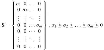
S=            

          

σ1 0 . . . 0 0 σ2. . . 0

..

. ... . .. ... 0 0 . . . σm 0 0 · · · 0

..

. ... . .. ... 0 0 . . . 0

           

          

, σ1≥σ2≥. . .≥σm≥0

Another way to write Eq. (1) is the so called spectral de-composition:

X= m X

i=1

σiuivTi (5)

where ui and vi are respectively U’s and V’s matrix i-th columns. But we had demonstrated that V=8, and from Eq. (1) it is not difficult to show that XV=US. So vi=8i andσiui=X8i where 8i is8’s i-th column. Substituting this equality in Eq. (5) permits us to obtain a simpler and more useful form for X’s decomposition:

X= m X

i=1

X8i8T_i (6)

2.2 Reconstruction stage

The aim of this stage is to separate the additive components of the time series. It can be seen as separating the time series into two groups: “our signal” and the “noisy” components, which are by definition the components we are not interested in.

The idea is to project the trajectory matrix over a q-dimensional space. In fact, in Eq. (5), every term of the sum has a lower importance with respect to the previous one in the construction of the signal. Such importance is given by the weightσiof each singular value of the base and σ1≥σ2≥. . .≥σm≥0 by construction. Then we can approxi-mate Eq. (5) and (6) with the following:

Xq= q X

i=1

σiuivTi (7)

and

noise= m X

i=q+1

σiuivTi (8)

or, in a simpler form:

Xq= q X

i=1

X8i8Ti (9)

and

noise= m X

i=q+1

X8i8T_i (10)

The criteria for this separation are not completely formalized and they depend on knowledge of the data, and obviously on σi’s modules. For example if the firstq singular values are much greater than the others, then the choice can be straight-forward.

The new matrix Xqis not always a trajectory matrix (be-cause in general it is not a Hankel matrix) and then it does not directly represent the noise-free x time series. However this time series can be obtained by a diagonal average method. For example, if Xqis the matrix:

Xq =    

  

x1,1x1,2x1,3 x2,1x2,2x2,3 x3,1x3,2x3,3 x4,1x4,2x4,3

   

  

then we obtain: xq=

n x1,1,

x2,1+x1,2

2 ,

x3,1+x2,2+x1,3

3 ,

x4,1+x3,2+x2,3

3 ,

x4,2+x3,3 2 , x4,3

o

In conclusion, the noise-free time series xqdepend on the choice of the parametersmandq, so we can write:

xq=SSA (x;m, q)

Obviously, the level of de-noising is higher whenqis lower. (Hegger et al., 1999) suggest thatqshould be at least the cor-rect embedding dimension, andmconsiderably larger (e.g. m=2qor larger).

3 Coupling of the singular values

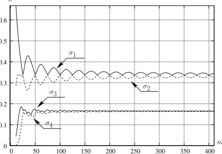
The behavior of the singular values (also called the spectrum of the singular values) can contain useful indications on the composition of the signal (i.e. Yang and Tse, 2003). In par-ticular, for a sufficiently high embedding dimension some of the singular values tend to show a certain degree of coupling, that isσ2→σ1,σ4→σ3and so on. An example is shown in Fig. 1. Note that in Fig. 1, the singular values are computed using the following definition of the covariance matrix:

C= 1

n−mX T_X

(4)

906 R. Carniel et al.: Singular values decoupling

Roberto Carniel et al.: Singular values decoupling 3

Another way to write Eq. (1) is the so called spectral de-composition:

X=

m X

i=1

σiuivTi (5)

where ui andvi are respectively U’s and V’s matrixi-th columns. But we had demonstrated that V =Φ, and from Eq. (1) it is not difficult to show thatXV=US. Sovi=Φi andσiui =XΦiwhereΦiisΦ’si-th column. Substituting this equality in Eq. (5) permits us to obtain a simpler and more useful form forX’s decomposition:

X=

m X

i=1

XΦiΦTi (6)

2.2 Reconstruction stage

The aim of this stage is to separate the additive components of the time series. It can be seen as separating the time series into two groups: “our signal” and the “noisy” components, which are by definition the components we are not interested in.

The idea is to project the trajectory matrix over a q -dimensional space. In fact, in Eq. (5), every term of the sum has a lower importance with respect to the previous one in the construction of the signal. Such importance is given by the weightσiof each singular value of the base and σ1 ≥ σ2 ≥ . . . ≥ σm ≥ 0by construction. Then we can approximate Eq. (5) and (6) with the following:

Xq= q X

i=1

σiuivTi (7)

and

noise= m X

i=q+1

σiuivTi (8)

or, in a simpler form:

Xq = q X

i=1

XΦiΦTi (9)

and

noise= m X

i=q+1

XΦiΦTi (10)

The criteria for this separation are not completely formalized and they depend on knowledge of the data, and obviously on σi’s modules. For example if the firstqsingular values are much greater than the others, then the choice can be straight-forward.

The new matrixXq is not always a trajectory matrix (be-cause in general it is not a Hankel matrix) and then it does not directly represent the noise-freextime series. However this time series can be obtained by a diagonal average method. For example, ifXqis the matrix:

Xq=       

x1,1x1,2x1,3

x2,1x2,2x2,3

x3,1x3,2x3,3

x4,1x4,2x4,3

      

then we obtain:

xq= n

x1,1,

x2,1+x1,2

2 ,

x3,1+x2,2+x1,3

3 ,

x4,1+x3,2+x2,3

3 ,

x4,2+x3,3 2 , x4,3

o

In conclusion, the noise-free time seriesxqdepend on the choice of the parametersmandq, so we can write:

xq=SSA(x;m, q)

Obviously, the level of de-noising is higher whenqis lower. (Hegger et al., 1999) suggest thatqshould be at least the cor-rect embedding dimension, andmconsiderably larger (e.g. m= 2qor larger).

3 Coupling of the singular values

The behavior of the singular values (also called the spectrum of the singular values) can contain useful indications on the composition of the signal (i.e. Yang and Tse (2003)). In par-ticular, for a sufficiently high embedding dimension some of the singular values tend to show a certain degree of coupling, that isσ2→σ1,σ4→σ3and so on. An example is shown in Fig. 1. Note that in Fig. 1, the singular values are computed using the following definition of the covariance matrix:

C= 1

n−mX T_X

In this way the singular values are detrended, allowing a sim-pler visualization. 0 0.1 0.2 0.3 0.4 0.5 0.6

0 50 100 150 200 250 300 350 400 σ

m

σ₃ σ2

σ₄ σ₁

Fig. 1. Example of coupling between singular values for the sig-nalsin (20·2πt) + 0.7 sin (57·2πt)(sampled at1000Hz) in an increasing embedding dimensionm= 10to400

We can define the“degree of coupling”as:

ρ1=

σ2

σ1

ρ2=

σ4

σ3 =. . .

ρk= σ2k σ2k−1

Fig. 1. Example of coupling between singular values for the signal

sin(20·2π t )+0.7 sin(57·2π t )(sampled at 1000 Hz) in an increas-ing embeddincreas-ing dimensionm=10 to 400.

4 Roberto Carniel et al.: Singular values decoupling

4 The data

One of the longest seismic time series available at Strom-boli comes from an automatic station installed in 1989 by the Dipartimento di Georisorse e Territorio of the University of Udine (Beinat et al., 1994) with the purpose of studying the long-term evolution of the strombolian activity (Carniel and Iacop, 1996a). The summit station, based on 3 Will-more MKIII/A seismometer (f0= 0.5Hz), is located at 800

m a.m.s.l. and at about 300 m from the craters (Beinat et al., 1994). During this last effusive phase, the hardware and soft-ware of the receiving station was upgraded in collaboration with CSIC, Madrid, for a continuous acquisition and internet data transmission. Data are now sampled with 16 bits (96dB) at 50 Hz (Ortiz et al., 2001; Carniel et al., 2006). Although at the time of 5 April 2003 paroxysmal event a dense network of monitoring equipment installed by the Civil Defence was operating, the explosion was not forecasted by any evident change in the data. In the following we will examine with the SSA methodology described above the seismic data recorded by our station during the days before this paroxysmal event, in particular from 25 March to 5 April 2003. The confidence in the method of analysis goes back again to Carniel et al. (2006), where another promising parameter was studied, de-rived from the SSA methodology:

rk= k X i=1 σi m X

i=k+1

σi

The idea behind this parameter was to monitor the time evo-lution of the relative weight of the firstkSSA components in the construction of the full tremor signal.

5 From tremor to singular values coupling

First of all we subdivide the raw data in windows of 60 s (i.e., 3000 sample points at 50 Hz). Both the methods of au-tocorrelation function and of mutual information (see 2.1.1) supply an embedding dimension estimatembetween 7 and 10, som = 10seems a correct minimal choice for the con-struction of the trajectory matrix. The singular values are computed on each of the one-minute time windows. In or-der to avoid amplitude-dependent effects, before the calcula-tion of the singular values, the data in each time window is normalized to zero mean and unitary variance. We start our analysis with the minimum embedding dimensionm= 10.

5.1 Behaviour ofρkparameter form= 10

We analyze the time evolution ofρkapproaching the

parox-ysmal event, that will be denoted by the hour "zero", at the extreme right of our graphs, for the embedding dimen-sionm = 10 (This embedding dimension is probably too small to capture the behaviour of the signal but allowed a

very fast analysis). The first two singular values do not show any anomalous behaviour in their ratioρ1, as can be

seen in Fig. 2. However, if we plot the same time evolu-tion but we take into account the“degree of coupling” be-tween the singular valuesσ3andσ4, i.e. ρ2, we observe a

very clear anomalous decrease of the parameter, that starts to diverge from the "normal" value - that theoretically, as we have shown, should be close to unity - already about 7 hours before the explosion (Fig. 3). Note that it is impor-tant to observe the relative change in the behaviour of the ρk rather than the absolute change. In fact, the coupling is

observed more easily for singular values of smaller indexes, while the phenomenon tends to be less evident as the index is increased. Moreover, the physical explanation of the cou-pling is still subject of research.

If we assume the lowest 5% percentile of the coupling pa-rameter range as a threshold for an alert, in this case the ab-solute value of the threshold is about 0.45. This threshold generates two short-lasting false alerts at about 115 and 152 hours before the explosion, but gives a "warning time" before the real explosion of more than6hours

0.3 0.4 0.5 0.6 0.7 0.8

−250 −200 −150 −100 −50 0 ρ₁

ratio

t[h]

Fig. 2.ρ1= σ_σ2₁in an embedding space of dimensionm= 10, for

Stromboli volcanic tremor

0.3 0.35 0.4 0.45 0.5 0.55

−250 −200 −150 −100 −50 0 ρ₂

t[h] ratio

threshold5%

false positive

Fig. 3.ρ2= σ_σ4

3in an embedding space of dimensionm= 10, for

Fig. 2. ρ1=σσ21 in an embedding space of dimension m=10, for

Stromboli volcanic tremor.

We can define the “degree of coupling” as: ρ1=

σ2 σ1

ρ2= σ4 σ3 =. . . ρk =

σ2k σ2k−1

4 The data

One of the longest seismic time series available at Strom-boli comes from an automatic station installed in 1989 by the Dipartimento di Georisorse e Territorio of the Univer-sity of Udine (Beinat et al., 1994) with the purpose of studying the long-term evolution of the strombolian activ-ity (Carniel and Iacop, 1996a). The summit station, based on

3 Willmore MKIII/A seismometer (f0=0.5 Hz), is located at 800 m a.m.s.l. and at about 300 m from the craters (Beinat et al., 1994). During this last effusive phase, the hardware and software of the receiving station was upgraded in col-laboration with CSIC, Madrid, for a continuous acquisition and internet data transmission. Data are now sampled with 16 bits (96 dB) at 50 Hz (Ortiz et al., 2001; Carniel et al., 2006). Although at the time of 5 April 2003 paroxysmal event a dense network of monitoring equipment installed by the Civil Defence was operating, the explosion was not fore-casted by any evident change in the data. In the following we will examine with the SSA methodology described above the seismic data recorded by our station during the days be-fore this paroxysmal event, in particular from 25 March to 5 April 2003. The confidence in the method of analysis goes back again to Carniel et al. (2006), where another promising parameter was studied, derived from the SSA methodology:

rk = k X

i=1 σi

m X

i=k+1 σi

5 From tremor to singular values coupling

First of all we subdivide the raw data in windows of 60 s (i.e., 3000 sample points at 50 Hz). Both the methods of autocor-relation function and of mutual information (see Sect. 2.1.1) supply an embedding dimension estimatembetween 7 and 10, so m=10 seems a correct minimal choice for the con-struction of the trajectory matrix. The singular values are computed on each of the one-minute time windows. In or-der to avoid amplitude-dependent effects, before the calcula-tion of the singular values, the data in each time window is normalized to zero mean and unitary variance. We start our analysis with the minimum embedding dimensionm=10. 5.1 Behaviour ofρkparameter form=10

(5)

R. Carniel et al.: Singular values decoupling 907

4 Roberto Carniel et al.: Singular values decoupling

4 The data

One of the longest seismic time series available at Strom-boli comes from an automatic station installed in 1989 by the Dipartimento di Georisorse e Territorio of the University of Udine (Beinat et al., 1994) with the purpose of studying the long-term evolution of the strombolian activity (Carniel and Iacop, 1996a). The summit station, based on 3 Will-more MKIII/A seismometer (f0= 0.5Hz), is located at 800

m a.m.s.l. and at about 300 m from the craters (Beinat et al., 1994). During this last effusive phase, the hardware and soft-ware of the receiving station was upgraded in collaboration with CSIC, Madrid, for a continuous acquisition and internet data transmission. Data are now sampled with 16 bits (96dB) at 50 Hz (Ortiz et al., 2001; Carniel et al., 2006). Although at the time of 5 April 2003 paroxysmal event a dense network of monitoring equipment installed by the Civil Defence was operating, the explosion was not forecasted by any evident change in the data. In the following we will examine with the SSA methodology described above the seismic data recorded by our station during the days before this paroxysmal event, in particular from 25 March to 5 April 2003. The confidence in the method of analysis goes back again to Carniel et al. (2006), where another promising parameter was studied, de-rived from the SSA methodology:

rk= k X i=1 σi m X

i=k+1 σi

5 From tremor to singular values coupling

First of all we subdivide the raw data in windows of 60 s (i.e., 3000 sample points at 50 Hz). Both the methods of au-tocorrelation function and of mutual information (see 2.1.1) supply an embedding dimension estimatembetween 7 and 10, som= 10seems a correct minimal choice for the con-struction of the trajectory matrix. The singular values are computed on each of the one-minute time windows. In or-der to avoid amplitude-dependent effects, before the calcula-tion of the singular values, the data in each time window is normalized to zero mean and unitary variance. We start our analysis with the minimum embedding dimensionm= 10.

5.1 Behaviour ofρkparameter form= 10

We analyze the time evolution ofρkapproaching the parox-ysmal event, that will be denoted by the hour "zero", at the extreme right of our graphs, for the embedding dimen-sionm = 10(This embedding dimension is probably too small to capture the behaviour of the signal but allowed a

very fast analysis). The first two singular values do not show any anomalous behaviour in their ratio ρ1, as can be

seen in Fig. 2. However, if we plot the same time evolu-tion but we take into account the“degree of coupling” be-tween the singular valuesσ3 andσ4, i.e. ρ2, we observe a

very clear anomalous decrease of the parameter, that starts to diverge from the "normal" value - that theoretically, as we have shown, should be close to unity - already about 7 hours before the explosion (Fig. 3). Note that it is impor-tant to observe the relative change in the behaviour of the ρk rather than the absolute change. In fact, the coupling is observed more easily for singular values of smaller indexes, while the phenomenon tends to be less evident as the index is increased. Moreover, the physical explanation of the cou-pling is still subject of research.

If we assume the lowest 5% percentile of the coupling pa-rameter range as a threshold for an alert, in this case the ab-solute value of the threshold is about 0.45. This threshold generates two short-lasting false alerts at about 115 and 152 hours before the explosion, but gives a "warning time" before the real explosion of more than6hours

0.3 0.4 0.5 0.6 0.7 0.8

−250 −200 −150 −100 −50 0 ρ₁

ratio

t[h]

Fig. 2.ρ1= σ_σ2

1 in an embedding space of dimensionm= 10, for

0.3 0.35 0.4 0.45 0.5 0.55

−250 −200 −150 −100 −50 0 ρ₂

t[h] ratio

threshold5%

false positive

Fig. 3.ρ2= σ_σ4

Fig. 3. ρ2=σσ43 in an embedding space of dimension m=10, for

from the “normal” value – that theoretically, as we have shown, should be close to unity – already about 7 h before the explosion (Fig. 3). Note that it is important to observe the relative change in the behaviour of theρkrather than the absolute change. In fact, the coupling is observed more easily for singular values of smaller indexes, while the phenomenon tends to be less evident as the index is increased. Moreover, the physical explanation of the coupling is still subject of re-search.

If we assume the lowest 5% percentile of the coupling pa-rameter range as a threshold for an alert, in this case the ab-solute value of the threshold is about 0.45. This threshold generates two short-lasting false alerts at about 115 and 152 h before the explosion, but gives a “warning time” before the real explosion of more than 6 hours

5.2 Behaviour ofρk parameter form>10

In order to verify that the anomalous behaviour is not strictly dependent on the particular choice of the embedding dimen-sionm=10, we performed a similar analysis also in higher dimensions, in particular form=20 andm=100. In both cases we observe again that some of the “degree of coupling” ratios show a strong decrease approaching the paroxysm. Figure 4 shows for instance the anomalous time behaviour of the ratioρ3=σ_σ6₅ in the embedding dimensionm=20, while Fig. 5 shows the anomalous decrease ofρ15=σ_σ30

29 in an em-bedding withm=100.

Using again the 5% percentile criterion, form=20 we have a threshold of about 0.75. As for the casem=10, we obtain false alerts at about 115 and 152 h before the true explosion. Also in this case however, the explosion is preceded by a warning more than 6 h in advance.

Form=100 the 5% percentile threshold corresponds to an absolute value of about 0.89. Also in this case we have false alerts at about 115 and 152 h before the true explosion, and an additional one about 48 h before the explosion.

5.2 Behaviour ofρkparameter form >10

In order to verify that the anomalous behaviour is not strictly dependent on the particular choice of the embedding dimen-sionm= 10, we performed a similar analysis also in higher dimensions, in particular for m = 20 andm = 100. In both cases we observe again that some of the"degree of cou-pling"ratios show a strong decrease approaching the parox-ysm. Fig. 4 shows for instance the anomalous time behaviour of the ratioρ3 = σσ65 in the embedding dimensionm= 20, while Fig. 5 shows the anomalous decrease ofρ15 = σσ3029 in an embedding withm= 100.

Using again the 5% percentile criterion, form = 20we have a threshold of about 0.75. As for the case m = 10, we obtain false alerts at about 115 and 152 hours before the true explosion. Also in this case however, the explosion is preceded by a warning more than6hours in advance.

Form= 100the 5% percentile threshold corresponds to an absolute value of about 0.89. Also in this case we have false alerts at about 115 and 152 hours before the true sion, and an additional one about 48 hours before the explo-sion. 0.5 0.55 0.6 0.65 0.7 0.75 0.8 0.85 0.9 0.95

−250 −200 −150 −100 −50 0

false positive threshold5%

ρ₃

t[h] ratio

Fig. 4.ρ3= σσ65in an embedding space of dimensionm= 20, for

0.76 0.78 0.8 0.82 0.84 0.86 0.88 0.9 0.92 0.94 0.96

−250 −200 −150 −100 −50 0

threshold5%

ρ₁₅

t[h] ratio

false positive

Fig. 5.ρ15= σ_σ30

29in an embedding space of dimensionm= 100,

for Stromboli volcanic tremor

6 Practical issues on the use of theρkparameter

Close to the paroxysmal event, as we have shown, only some of theρk parameters show an anomalous decreasing

behaviour. Otherρk on the contrary don’t show anything

interesting. Consequently, a problem arises regarding the number of parameters to be monitored in order to observe possible anomalous behavior. We propose here a solution to this problem, with the definition of a "summarizing" param-eter defined as the minimum of allρk computed in a given

embedding dimension. Care should be taken however in or-der to obtain meaningful results: the last ratios should be excluded from this minimum calculation. The last (i.e. the least important) components of the SSA decomposition are in fact associated to what is essentially a noise signal (8), and should therefore be removed. We can then finally define:

ˆ

ρq= min

k=1..q{ρk−µk} q < m

whereµkis the average of the ratioρkthat can be estimated

during a normal period of activity (in our case the first 4 days in the graph). A suitable value ofqshould be chosen; a rule of thumb is to take

q'1 3m

In Fig. 6 the time evolution of the parameterρˆqis shown for q= 4in an embedding dimensionm= 20. The decreasing anomalous behaviour is again very evident before the parox-ysmal event.

−250 −200 −150 −100 −50 −0 −0.30 −0.25 −0.20 −0.15 −0.10 −0.05 0.00 0.05 ratio ˆ ρ₄ t[h] threshold5%

Fig. 6.ρˆ4in an embedding space of dimensionm= 20, for

Strom-boli volcanic tremor

In Fig. 4 a phase is evident with a peculiar behaviour start-ing about 40 hours before the explosion. This is the time at which Carniel et al. (2006) observe the first successful ap-plication of the Failure Forecast Method (FFM), that gives a forecast for 5 April 2003 at 15 GMT (see line 1 in Fig. 9 of Carniel et al. (2006)). More than 6 hours before the explo-sion, theρ2,ρ4,ρ15andρˆ4parameters (see Fig. 3, 4, 5 and 6

respectively) go below the percentile threshold of 5%. At this time the FFM (see line 2 in Fig. 9 in Carniel et al. (2006)), af-ter an apparent recovery of the stability, is able again to give Fig. 4. ρ3=σσ65 in an embedding space of dimension m=20, for

In order to verify that the anomalous behaviour is not strictly dependent on the particular choice of the embedding dimen-sionm= 10, we performed a similar analysis also in higher dimensions, in particular for m = 20 andm = 100. In both cases we observe again that some of the"degree of cou-pling"ratios show a strong decrease approaching the parox-ysm. Fig. 4 shows for instance the anomalous time behaviour of the ratioρ3 = σ_σ6₅ in the embedding dimensionm= 20,

while Fig. 5 shows the anomalous decrease ofρ15 = σ_σ30₂₉ in

an embedding withm= 100.

Using again the 5% percentile criterion, form = 20we have a threshold of about 0.75. As for the casem = 10, we obtain false alerts at about 115 and 152 hours before the true explosion. Also in this case however, the explosion is preceded by a warning more than6hours in advance.

Form= 100the 5% percentile threshold corresponds to an absolute value of about 0.89. Also in this case we have false alerts at about 115 and 152 hours before the true sion, and an additional one about 48 hours before the explo-sion. 0.5 0.55 0.6 0.65 0.7 0.75 0.8 0.85 0.9 0.95

−250 −200 −150 −100 −50 0

ρ₃

t[h] ratio

Fig. 4.ρ3= σ_σ6

0.76 0.78 0.8 0.82 0.84 0.86 0.88 0.9 0.92 0.94 0.96

−250 −200 −150 −100 −50 0

threshold5%

ρ₁₅

t[h] ratio

false positive

Fig. 5.ρ15= σ_σ30

29 in an embedding space of dimensionm= 100,

Close to the paroxysmal event, as we have shown, only some of theρk parameters show an anomalous decreasing behaviour. Otherρk on the contrary don’t show anything interesting. Consequently, a problem arises regarding the number of parameters to be monitored in order to observe possible anomalous behavior. We propose here a solution to this problem, with the definition of a "summarizing" param-eter defined as the minimum of allρk computed in a given embedding dimension. Care should be taken however in or-der to obtain meaningful results: the last ratios should be excluded from this minimum calculation. The last (i.e. the least important) components of the SSA decomposition are in fact associated to what is essentially a noise signal (8), and should therefore be removed. We can then finally define:

ˆ

ρq = min

whereµkis the average of the ratioρkthat can be estimated during a normal period of activity (in our case the first 4 days in the graph). A suitable value ofqshould be chosen; a rule of thumb is to take

q' 1 3m

In Fig. 6 the time evolution of the parameterρqˆ is shown for q = 4in an embedding dimensionm= 20. The decreasing anomalous behaviour is again very evident before the parox-ysmal event.

−250 −200 −150 −100 −50 −0 −0.30 −0.25 −0.20 −0.15 −0.10 −0.05 0.00 0.05 ratio ˆ ρ₄ t[h] threshold5%

respectively) go below the percentile threshold of 5%. At this time the FFM (see line 2 in Fig. 9 in Carniel et al. (2006)), af-ter an apparent recovery of the stability, is able again to give Fig. 5. ρ15=σσ3029 in an embedding space of dimensionm=100, for

6 Practical issues on the use of theρkparameter Close to the paroxysmal event, as we have shown, only some of theρk parameters show an anomalous decreasing behaviour. Other ρk on the contrary don’t show anything interesting. Consequently, a problem arises regarding the number of parameters to be monitored in order to observe possible anomalous behavior. We propose here a solution to this problem, with the definition of a ”summarizing” param-eter defined as the minimum of allρk computed in a given embedding dimension. Care should be taken however in or-der to obtain meaningful results: the last ratios should be excluded from this minimum calculation. The last (i.e. the least important) components of the SSA decomposition are in fact associated to what is essentially a noise signal (8), and should therefore be removed. We can then finally define:

ˆ

ρq = min k=1..q

{ρk−µk} q < m

(6)

908 R. Carniel et al.: Singular values decoupling

In order to verify that the anomalous behaviour is not strictly dependent on the particular choice of the embedding dimen-sionm= 10, we performed a similar analysis also in higher dimensions, in particular form = 20and m = 100. In both cases we observe again that some of the"degree of cou-pling"ratios show a strong decrease approaching the parox-ysm. Fig. 4 shows for instance the anomalous time behaviour of the ratioρ3 = σ_σ6₅ in the embedding dimensionm= 20,

while Fig. 5 shows the anomalous decrease ofρ15 =σ_σ30₂₉ in

an embedding withm= 100.

Using again the 5% percentile criterion, form= 20we have a threshold of about 0.75. As for the casem = 10, we obtain false alerts at about 115 and 152 hours before the true explosion. Also in this case however, the explosion is preceded by a warning more than6hours in advance.

Form= 100the 5% percentile threshold corresponds to an absolute value of about 0.89. Also in this case we have false alerts at about 115 and 152 hours before the true sion, and an additional one about 48 hours before the explo-sion.

0.5 0.55 0.6 0.65 0.7 0.75 0.8 0.85 0.9 0.95

−250 −200 −150 −100 −50 0

ρ₃

t[h] ratio

Fig. 4.ρ3= σ_σ6

5in an embedding space of dimensionm= 20, for

0.76 0.78 0.8 0.82 0.84 0.86 0.88 0.9 0.92 0.94 0.96

−250 −200 −150 −100 −50 0

threshold5%

ρ₁₅

t[h] ratio

false positive

Fig. 5.ρ15= σ_σ30

29in an embedding space of dimensionm= 100,

Close to the paroxysmal event, as we have shown, only some of the ρk parameters show an anomalous decreasing behaviour. Other ρk on the contrary don’t show anything interesting. Consequently, a problem arises regarding the number of parameters to be monitored in order to observe possible anomalous behavior. We propose here a solution to this problem, with the definition of a "summarizing" param-eter defined as the minimum of allρk computed in a given embedding dimension. Care should be taken however in or-der to obtain meaningful results: the last ratios should be excluded from this minimum calculation. The last (i.e. the least important) components of the SSA decomposition are in fact associated to what is essentially a noise signal (8), and should therefore be removed. We can then finally define:

ˆ

ρq= min

whereµkis the average of the ratioρkthat can be estimated during a normal period of activity (in our case the first 4 days in the graph). A suitable value ofqshould be chosen; a rule of thumb is to take

q' 1 3m

In Fig. 6 the time evolution of the parameterρqˆ is shown for q = 4in an embedding dimensionm= 20. The decreasing anomalous behaviour is again very evident before the parox-ysmal event.

−250 −200 −150 −100 −50 −0 −0.30

−0.25 −0.20 −0.15 −0.10 −0.05 0.00 0.05 ratio

ˆ

ρ₄

t[h] threshold5%

respectively) go below the percentile threshold of 5%. At this time the FFM (see line 2 in Fig. 9 in Carniel et al. (2006)), af-ter an apparent recovery of the stability, is able again to give Fig. 6.ρˆ4in an embedding space of dimensionm=20, for Stromboli

volcanic tremor.

in the graph). A suitable value ofq should be chosen; a rule of thumb is to take

q '1 3m

In Fig. 6 the time evolution of the parameter ρˆq is shown forq=4 in an embedding dimensionm=20. The decreasing anomalous behaviour is again very evident before the parox-ysmal event.

In Fig. 4 a phase is evident with a peculiar behaviour start-ing about 40 hours before the explosion. This is the time at which Carniel et al. (2006) observe the first successful ap-plication of the Failure Forecast Method (FFM), that gives a forecast for 5 April 2003 at 15 GMT (see line 1 in Fig. 9 of Carniel et al. (2006)). More than 6 h before the explosion, the ρ2,ρ4,ρ15andρˆ4parameters (see Fig. 3, 4, 5 and 6, respec-tively) go below the percentile threshold of 5%. At this time the FFM (see line 2 in Fig. 9 in Carniel et al. (2006)), after an apparent recovery of the stability, is able again to give a (even more reliable) forecast, for 5 April 2003 at 10:20 GMT, with a less than 3 h difference with respect to the real occurrence of the explosion.

A practical problem is that there are some embedding di-mension ranges for which the anomalous behaviour disap-pears. One can think of a minimization procedure similar to the one adopted for the index of the ratio, but exploring e.g. every embedding dimension in the rangem=10 to 500, al-though theoretically possible, can lead to unacceptable com-puting times.

Also the choice of the minimum embedding dimension to use is not straightforward. The value suggested by the first zero of the autocorrelation function or by the first minimum of the mutual information (i.e.m=10) seems in fact too low.

7 Conclusions

Forecasting paroxysmal events such as the one recorded on Stromboli on 5 April 2003 is of paramount importance, es-pecially at a volcano like Stromboli, where tourism is a ma-jor economical resource. This is undoubtly a difficult task if we consider the forecast in a deterministic sense. How-ever, if we consider the risk of a volcano in a probabilistic sense (Aspinall et al., 2003, 2005) the issuing of a Tempo-rary Increase in Probability of a paroxysmal event would be already a considerable success. In order to do this, a num-ber of parameters should be monitored and their anomalies highlighted and weighted in a bayesian sense. Different use-ful parameters can be derived from the Singular Spectrum Analysis, one of which – therkparameter weighting the rel-ative importance of the firstkSSA components in the con-struction of a geophsyical signal – was proposed by Carniel et al. (2006). In this paper we have shown the potential of another family of parameters,ρk, which measure the degree of coupling between successive singular values. A practical way of getting rid of the problem of how to choose which of these couplings to monitor was also proposed, with the parameterρˆq, which looks for the (significant) minimum of these degrees of coupling. An important brand new class of monitoring parameters are therefore available for inclusion in bayesian eruptive scenario evaluators. Obviously, further (and possibly forward) testing on other cases is needed for testing the effective forecasting capabilities of these new pa-rameters.

Acknowledgements. The methodologies developed and applied in this work are partially supported by the projects “V4 – Conception, verification and application of innovative techniques for studying volcanoes” by the Istituto Nazionale di Geofisica e Vulcanologia – Dipartimento Protezione Civile, Italy, “TEGETEIDE – Técnicas geofísicas y geodésicas para el estudio de la zona volcánica activa del complejo Teide – Pico Viejo (Tenerife)”, Spain, TEI-DEVS (Spain, CGL2004-05744), INGV-DPC V4 “Conception, verification, and application of innovative techniques to study active volcanoes” (Italy) and PRIN 2004131177 “Numerical and graphical methods for the analysis of time series data” (Italy). The SCILAB package (see http://www.scilab.org) was used to integrate the different analysis routines. Italian Civil Defence provided logistic support when access to the summit area was forbidden. The seismic station was originally installed under a research grant of the Italian Gruppo Nazionale di Vulcanologia. The authors gratefully acknowledge the collaboration of J. Alean, S. Ballarò, S. Calvari, C. Cardaci, M. Fulle, A. García, A. Llinares, P. Malisan, V. Perin, M. Ripepe and three anonymous referees in the various stages of data acquisition, logistic help, data analysis, interpretation and manuscript reviewing.

(7)

R. Carniel et al.: Singular values decoupling 909 References

Aldrich, C. and Barkhuizen, M.: Process system identification strategies based on the use of singular spectrum analysis, Min-erals Engineering, 16, 815–826, 2003.

Alean, J., Carniel, R., and Fulle, M.: Stromboli online, volcanoes of the world: Information on Stromboli, Etna and other volcanoes, http://stromboli.net, 2006.

Aspinall, W., Woo, G., Voight, B., and Baxter, J.: Evidence-based volcanology: application to eruption crises, Journal of Volcanol-ogy and Geothermal Research, 128, 273–285, 2003.

Aspinall, W., Carniel, R., Hincks, T., Jaquet, O., and Woo, G.: Using Hidden Multi-state Markov models with multi-parameter volcanic data to provide empirical evidence for alert level decision-support, Journal of Volcanology and Geothermal Re-search, 153, 112–124, 2005.

Barberi, F., Rosi, M., and Sodi, A.: Volcanic hazard assessment at Stromboli based on review of historical data, Acta Vulcanolog-ica, 3, 173–187, 1993.

Beinat, A., Carniel, R., and Iacop, F.: Seismic station of Strom-boli: 3-component data acquisition system, Acta Vulcanologica, 5, 221–222, 1994.

Broomhead, D. and King, G.: Extracting qualitative dynamics from experimental data, Phisica, D(20), 217–236, 1981.

Calvari, S.: Stromboli report, Bulletin Global Volcanism Network, Smithsonian Institution, Smithsonian Institution, 28, 8, 5–5, 2003.

Carniel, R. and Di Cecca, M.: Dynamical tools for the analysis of long term evolution of volcanic tremor at Stromboli, Annali di Geofisica, 42, 3, 483–495, 1999.

Carniel, R. and Iacop, F.: On the persistency of crater assignment criteria for Stromboli explosion-quakes, Annali di Geofisica, 39, 2, 347–359, 1996a.

Carniel, R. and Iacop, F.: Spectral precursors of paroxysmal phases of Stromboli, Annali di Geofisica, 39, 2, 327–345, 1996b. Carniel, R., Di Cecca, M., and Rouland, D.: Ambrym, Vanuatu

(July-August 2000): Spectral and dynamical transitions on the hours-to-days timescale, Journal of Volcanology and Geothermal Research, 128, 1-3, 1–13, 2003.

Carniel, R., Ortiz, R., and Di Cecca, M.: Spectral and dynamical hints on the timescale of preparation of the 5 April 2003 explo-sion at Stromboli volcano, Can. J. Earth Sci. , 43, 41–55, 2006. Francalanci, L., Tommasini, S., and Conticelli: The volcanic

ac-tivity of Stromboli in the 1906–1998 AD period: mineralogical, geochemical and isotope data relevant to the understanding of the plumbing system, Journal of Volcanology and Geothermal Research, 131, 179–211, 2004.

Fraser, A.: Using mutual information to estimate metric entropy in Dimensions and Entropies in Chaotic Systems, Springer Verlag, 82–91, 1986.

Fraser, A. and Swinney, H.: Independent coordinates for strange attractors from mutual information, Phis.Rev. A., 33(2), 1134– 1140, 1986.

Golyandina, N., Nekrutkin, V., and Zhigljavsky, A.: Analysis of time series structure-SSA and related techniques, Chapman & Hall/CRC, 2001.

Harris, A., Carniel, R., and Jones, J.: Identification and Modelling of Variable Convective Regimes at Erta Ale lava lake, Journal of Volcanology and Geothermal Research, 142, 3–4, 207–223, 2005.

Hegger, R., Kantz, H., and Schreiber, T.: Practical implementa-tion of nonlinear time series methods: The TISEAN package, CHAOS, 9, 413–435, 1999.

Jaquet, O. and Carniel, R.: Stochastic modelling at Stromboli: a volcano with remarkable memory, Journal of Volcanology and Geothermal Research, 105, 249–262, 2001.

Jaquet, O. and Carniel, R.: Multivariate stochastic modelling: towards forecasts of paroxysmal phases at Stromboli, Journal of Volcanology and Geothermal Research, 128, 1–3, 261–271, 2003.

Jones, J., Carniel, R., Malone, S., and Harris, A.: Seismic charac-teristics of variable convection at Erta Ale lava lake, Ethiopia, Journal of Volcanology and Geothermal Research, 153, 64–79, 2005.

Konstantinou, K. and Schlindwein, V.: Nature, wavefield properties and source mechanisms of volcanic tremor: a review, Journal of Volcanology and Geothermal Research, 119, 161–187, 2002. Marelli, L., Bilato, R., Franz, P., Martin, P., Murai, A., and

O’Gorman, M.: Singular spectrum analysis as a tool for plasma fluctuation analysis, Review of Scientific Instruments, 72(1), 499–502, 2002.

Mineva, A. and Popivanov, D.: Method for single-trial readiness po-tential identification, based on singular spectrum analysis, Jour-nal of Neuroscience Method, 68, 91–99, 1996.

Ortiz, R., García, A., and Astiz, M.: Instrumentación en Vol-canología, Servicio de Publicaciones del Cabildo Insular de Lan-zarote, 345, 2001.

Pereira, W. and Maciel, C.: Performance of ultrasound echo de-composition using singular spectrum analysis, Ultrasound in Medicine and Biology, 27(9), 1231–1238, 2001.

Ripepe, M., Harris, A., and Carniel, R.: Thermal, seismic and infra-sonic evidences of variable degassing rates at Stromboli volcano, Journal of Volcanology and Geothermal Research, 118, 285–297, 2002.

Rosi, M., Bertagnini, A., and Landi, P.: Onset of the persistent ac-tivity at Stromboli Volcano (Italy), Bulletin of Volcanology, 62, 294–300, 2000.

Shaw, R.: The Dripping Faucet as a Model Chaotic System, Aerial Press, Santa Cruz, CA., 2000.

Takens, F.: Detecting strange attractor in turbulence, Lecture Notes in Math, 898, 366–381, 1981.