Nat. Hazards Earth Syst. Sci., 11, 3327–3334, 2011 www.nat-hazards-earth-syst-sci.net/11/3327/2011/ doi:10.5194/nhess-11-3327-2011
© Author(s) 2011. CC Attribution 3.0 License.
Natural Hazards
and Earth
System Sciences
About the influence of elevation model quality and small-scale
damage functions on flood damage estimation
M. Boettle, J. P. Kropp, L. Reiber, O. Roithmeier, D. Rybski, and C. Walther
Potsdam Institute for Climate Impact Research, 14412 Potsdam, Germany
Received: 21 February 2011 – Revised: 28 July 2011 – Accepted: 4 October 2011 – Published: 19 December 2011
Abstract. The assessment of coastal flood risks in a particu-lar region requires the estimation of typical damages caused by storm surges of certain characteristics and annualities. Al-though the damage depends on a multitude of factors, includ-ing flow velocity, duration of flood, precaution, etc., the rela-tionship between flood events and the corresponding average damages is usually described by a stage-damage function, which considers the maximum water level as the only dam-age influencing factor. Starting with different (microscale) building damage functions we elaborate a macroscopic dam-age function for the entire case study area Kalundborg (Den-mark) on the basis of multiple coarse-graining methods and assumptions of the hydrological connectivity. We find that for small events, the macroscopic damage function mostly depends on the properties of the elevation model, while for large events it strongly depends on the assumed building damage function. In general, the damage in the case study increases exponentially up to a certain level and then less steep.
1 Introduction
In order to estimate the damage costs of future storm surges one can apply the concept of stage-damage functions (see e.g. Smith, 1994) which provide for a flood of certain water level a corresponding direct monetary damage. Combined with extreme value statistics, the risk can be calculated. Both components, extreme value statistics and damage functions, involve uncertainties (Merz and Thieken, 2004; Merz et al., 2004) and crucially influence the outcome (Merz et al., 2002; Apel et al., 2009).
Correspondence to: M. Boettle
A macroscopic stage-damage function (i.e. a function that represents the total damage in the entire considered area) can be obtained by summing up all damages of a lower scale (e.g. building scale) or by an indirect approach (Steinh¨auser et al., 2011). Here we follow the former approach to assess the macroscopic damage function of a case study area in Den-mark. For this purpose it is necessary to determine the in-undation height of each asset (e.g. building) for certain flood events in order to calculate the corresponding damage. Since hydrodynamic modelling requires more effort and computa-tional power, many studies use a simple flood fill algorithm, i.e. they determine the intersection between the plane of the raised water level and the digital elevation model (DEM), and treat the entire connected area between sea and intersection as inundated (Dasgupta et al., 2008; Mazria and Kershner, 2007; Rowley et al., 2007). This procedure overestimates the flooded area since it corresponds to an asymptotic filling of all land that would be flooded at a certain permanent sea level.
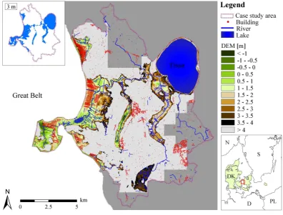
Fig. 1. Map of the case study area and location within Northern Europe. The elevation according to the available DEM is colour coded (light
grey represents elevations above4m) and buildings are indicated by red dots. The dark grey area delineates land for which no elevation data is available and the white area in the east is the sea. The inset in the upper left corner indicates the inundated area for a 3 m sea level referred to DVR90 (no aggregation, 4 nearest neighbours). The inset in the lower right shows the country contours and the cut-out representing the major map. DEM owned by BlomInfo A/S, Denmark.
0 1 2 3
water level [m] 0
0.2 0.4 0.6
building damage fraction
square root linear quadratic
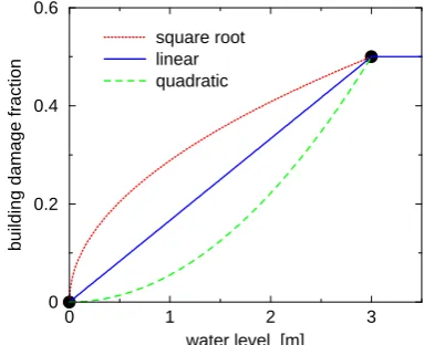
Fig. 2. Assumed building damage functions according to Eqs. (1),
(3), and (4). The fraction of building damage (without inventory) is plotted against the water level from the lower edge of the building. The parameters of the linear, square root, and quadratic building damage function are determined by two anchor points, i.e. no dam-age for no inundation and 50% damdam-age at3m inundation.
nearest neighbours nearest and 2nd
nearest neighbours
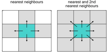
Fig. 3. Illustration of inundation via 4 nearest (left) or 8 nearest
(right) neighbours. The former uses only nearest neighbours, i.e. at cell distance1, the latter also includes second nearest neighbours,
i.e. at cell distance√2.
Fig. 1. Map of the case study area and location within Northern Europe. The elevation according to the available DEM is colour coded (light
grey represents elevations above 4 m) and buildings are indicated by red dots. The dark grey area delineates land for which no elevation data is available and the white area in the east is the sea. The inset in the upper left corner indicates the inundated area for a 3 m sea level referred to DVR90 (no aggregation, 4 nearest neighbours). The inset in the lower right shows the country contours and the cut-out represents the major map. DEM owned by BlomInfo A/S, Denmark.
neighbours (this represents different assumptions about the hydrological connectivity according to Poulter and Halpin, 2008). (ii) Coarse-graining (aggregating) the DEM in 2 by 2 cells or 3 by 3 cells (or no coarse-graining). (iii) Using the minimum, mean, or maximum within the coarse-grained cells. Furthermore, we base our calculations on linear, square root, or quadratic building damage functions.
We find that all macroscopic damage functions can be characterised by three regimes: a zero level for moderate wa-ter levels followed by an exponential and a less steep increase for high water levels. Moreover, we show that the inundation mode is the most dominant factor for the damage estimation of small events, whereas the choice of the building damage function is dominating for heavy floodings.
In Sect. 2 we provide information about the case study and the data used. The performed analysis is described in Sect. 3 and the obtained results are presented in Sect. 4. We sum-marise and draw conclusions in Sect. 5.
2 Case study area
The case study area (displayed in Fig. 1) is situated in the south of the city of Kalundborg in Denmark. The considered area belongs to the municipality of Kalundborg which itself is located on the west coast of the island of Zealand. To the west, the case study area borders at the Jammerland Bay, the Musholm Bay, and the Great Belt which connects the Baltic Sea with the marine area Kattegat. There are a few small rivers and the fourth-largest lake of Denmark, Lake Tissø, in the area.
M. Boettle et al.: Influence of elevation model quality and small-scale damage functions 3329 with a vertical resolution of 10 cm. The region is
predom-inantly rather flat with a range in elevation of almost 55 m. However, some areas lie below sea level (approx. 0.9 km2).
The case study area contains more than 6000 properties with almost 17 000 structures concentrated in a few settle-ments with approx. 200 to 4500 inhabitants. The cadastral dataset contains information about the building position, type of the building, property value and land value but not about the size and shape of the structures. This implies, that the flood flow procedure cannot consider the buildings as barri-ers, which is only a minor limitation, since most buildings stand separately and are not adjacent. Property and land value were obtained from the calculation basis for property taxes and were provided by the municipality. Their differ-ence leads to the building value, which was used to estimate building damages in combination with relative stage-damage functions.
The buildings are grouped into six main types: garages, carports etc. (42 %); year-round residential (25 %); recre-ational purposes (18 %); agriculture, industry etc. (13 %); trade, transport etc. (1 %); (social) institutions (1 %). Ac-cordingly, the case study area is characterized by small lo-calities, a low population density, many summer cottages, agriculture, and minor industry.
3 Analysis
In the performed analysis, we focus on a hypothetical storm surge event of certain levelE(referred to DVR90) and as-sume that the sea water completely inundates the terrain at this considered water level. Thus, we disregard the dynamics and study an asymptotic static inundation scenario; it does not take into account any decline in flood level and volume with increasing distance from the coast. Accordingly, the in-undated area is defined as the connected area between the sea and the intersection of the raised water level and the elevation model.
In order to identify the inundated area, we start from a cell that is clearly located in the sea. Then we check if the neighbouring cells have an elevation below the chosen sea level (this is true for cells belonging to the sea). If this is the case, we mark it as inundated and proceed with its neigh-bouring cells. This procedure is continued until all adjacent cells below the chosen level are identified. Please note, that low lying areas that are not connected are not included.
In the next step, we determine which of the properties are within the inundated area and calculate how deep each ing is flooded. Since the available dataset locates each build-ing to a grid cell in the DEM, representbuild-ing the centre of the building, the correspondig elevation is assigned to the struc-ture. The buildings have no cellar and a typical foundation base of 20 cm above which we estimate the damage for indi-vidual buildings as a fraction of their value.
0 1 2 3
water level [m] 0
0.2 0.4 0.6
building damage fraction
square root linear quadratic
Fig. 2. Assumed building damage functions according to Eqs. (1),
(3), and (4). The fraction of building damage (without inventory) is plotted against the water level from the lower edge of the building. The parameters of the linear, square root, and quadratic building damage function are determined by two anchor points, i.e. no dam-age for no inundation and 50 % damdam-age at 3 m inundation.
A wide range of functional forms, such as logarithmic, square-root, linear and quadratic (see Nascimento et al., 2007; Dutta et al., 2003; B¨uchele et al., 2006; Apel et al., 2009, and references therein) have been used as building damage functions in previous studies. To exemplify our ap-proach, we choose a linear function
dlin(e)=
0 fore <0 m e
3 m0.5 for 0 m≤e≤3 m
0.5 fore >3 m
, (1)
wheree denotes the water level relative to the foundation base of the building (see Fig. 2).
This is done for all affected buildings and the total damage for the considered sea levelEis calculated as
Dlin(E)=
X
i
dlin(ei)Vi , (2)
whereei is the flood height at buildingi andVi its value. We considerD(E)as an estimate of the total monetary dam-age (without inventory) caused by a certain flood of levelE to the buildings in the entire case study area. By varying the sea levelE in steps of 10 cm between 0 m and 3 m we obtain a macroscopic damage function. Based on sea level records, provided by the municipality of Kalundborg, a 3 m storm surge corresponds approx. to a 800-yr event (the upper left inset of Fig. 1 depicts a 3 m flood).
Table 1. Overview of the explored inundation determination modes
sorted by the estimated damage (high damage from top) along with the lowest water level, for which a considerable damage (over 1 mil-lion DKK) is found (last column). The options differ in the number of nearest neighbours considered (2nd column), the coarse-graining (3rd column), and the value associated to the coarse-grained cells (4th column), see Sect. 3.
rank neighbours coarse aggregation first graining mode considerable damage 1. 8 3×3 min 60 cm 2. 4 3×3 min 110 cm 3. 8 2×2 min 110 cm 4. 4 2×2 min 110 cm 5. 8 3×3 mean 120 cm 6. 4 3×3 mean 120 cm 7. 8 2×2 mean 130 cm 8. 4 2×2 mean 130 cm
9. 8 – – 140 cm
10. 4 – – 140 cm
11. 8 2×2 max 140 cm 12. 4 2×2 max 140 cm 13. 8 3×3 max 140 cm 14. 4 3×3 max 150 cm
1. Inundation via 4 or 8 adjacent cells
In the above described procedure the inundated area is identified by checking whether neighbouring cells have an elevation below certain threshold. Since the inunda-tion might not only propagate to the east, north, west, and south, but also in diagonal direction, we test these two options. As illustrated in Fig. 3 either the 4 or 8 nearest cells are considered as adjacent. This means in the latter case also the second nearest neighbours are included.
2. Resolution of the Digital Elevation Model (no coarse-graining, 2×2, or 3×3 cells)
Since each DEM has a limited horizontal resolution, we test by coarse-graining (i.e. aggregation) how sensitive the result responds to the resolution of the data. The available DEM can be considered as a coarse-grained DEM from an even higher resolution. In many areas only low resolution DEM are available.
3. Minimum, mean, or maximum coarse-graining
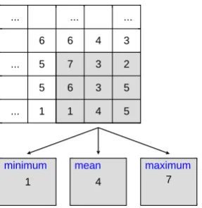
When coarse-graining, we elaborate three options of as-sociating an elevation value to the new aggregated cells, as illustrated in Fig. 4. These options specify, whether we assume that the flood is strong enough to overtop or break through higher elevated areas. In a sense, these options correspond to worst and best case scenarios.
nearest neighbours nearest and 2nd
nearest neighbours
Fig. 3. Illustration of inundation via 4 nearest (left) or 8 nearest
(right) neighbours. The former uses only nearest neighbours, i.e. at cell distance 1, the latter also includes second nearest neighbours, i.e. at cell distance
√
2.
4. Linear, square root, or quadratic building damage func-tion
As mentioned above, many different building damage functions are proposed and used in the literature. We study the influence of a linear, Eq. (1), a square root,
dsqrt(e)=
0 fore <0 m (3 me )1/20.5 for 0 m≤e≤3 m 0.5 fore >3 m
, (3)
and a quadratic,
dquad(e)=
0 fore <0m (3 me )20.5 for 0 m≤e≤3 m 0.5 fore >3 m
, (4)
functional form on the final macroscopic damage func-tion. As can be confirmed with Fig. 2, the parameters have been chosen so that there is no damage if the build-ing is not flooded and a maximum damage of 50 % when the building is flooded by 3 m or more. Of course these two points influence the final results but our major find-ings are independent of their actual values.
We end up with 14 combinations (modes) of determining the inundated area and building inundation for each of the three damage functions.
4 Results
Beginning with the linear building damage function, Eq. (1), we obtain a variety of different macroscopic damage func-tions which are displayed in Fig. 5. Different things can be observed:
M. Boettle et al.: Influence of elevation model quality and small-scale damage functions 3331
7 3 2
6 3 5
1 4 5
1 5 5
6 6 4 3
... ... ...
...
...
1
minimum
7
maximum
4
mean
Fig. 4. Illustration of coarse-graining modes of the elevation model
employing minimum, mean, and maximum. For an aggregation of 3×3 grid cells in the DEM (top) an example of the different result-ing cell values (bottom) is displayed (with exemplary numbers).
2. At low sea levels around 1–1.5 m the damage increases abruptly from zero to the order of 10 million Danish Krones (DKK).
3. The damage increases exponentially up to 2–2.5 m above which it follows a less steep function.
4. The damages for all inundation modes at intermediate and high sea levels range approx. 10 %.
The abrupt increase in the macroscopic damage is a natu-ral effect to be expected. Once the sea level exceeds natunatu-ral or artificial barriers in the DEM, the entire area behind is considered as inundated. In this context, a barrier is a set of grid cells, that is higher elevated than the water level and that is located in a way, such that the water cannot flow around. However, at which sea level such a step occurs depends on the applied inundated mode. Already at 60 cm a damage of approx. 6 million DKK is found in the case of 3×3, mini-mum, 8 neighbours. In the best case, the first considerable damage (over 1 million DKK) occurs at 1.5 m with approx. 29 million DKK (3×3, maximum, 4 neighbours). The water levels, at which this jump occurs in each inundation mode are listed in Table 1.
In addition, Table 1 ranks all combinations according to their damage. It is apparent, that taking the minimum in the coarse-graining leads always to larger damages and taking the maximum leads to smaller damages. This is clear, be-cause possible barriers as well as buildings are lowered or raised. In addition, this effect is more pronounced for coarse-graining in 3×3 than in 2×2 cells.
We would like to note that in practice coarse-graining tak-ing the mean value is the relevant mode. If we compare the damage functions from the coarse grained and non-coarse-grained DEM, we find that the damage range for high wa-ter levels is approximately constant, which implies that the relative difference becomes insignificant. For the damage
0 1 2 3
water level [m] 0
100 200 300 400 500
damage [million DKK]
0 1 2 3
10−3
10−2
10−1
100
101
102
103
Fig. 5. Macroscopic damage function for different modes of
in-undation determination. The estimated direct monetary damage is plotted against the water level for the following variations as de-tailed in Table 1 (top to bottom). (i) Considering 4 or 8 nearest neighbours is represented by a solid or dotted line. (ii) Coarse-graining in 2×2 cells or 3×3 cells is represented by orange or green (no coarse-graining: black). (iii) The width of the lines rep-resents the value associated to the coarse grained cells: minimum – thin, mean – medium, maximum – thick. A linear building damage function according to Eq. (1) has been used, see Fig. 2. The inset shows the same curves but in semi-logarithmic scale.
determination of severe events the resolution of the DEM is therefore of minor importance. This can be explained by the fact that for high water levels the buildings are flooded more deeply and the error caused by coarse-graining there-fore becomes less important. However, for low flood levels, the abrupt jumps in the functions can lead to large differ-ences for singular levels, usually with larger damage in the coarse-grained cases. Hence, the quality of the DEM is deci-sive for the damage determination of small events. Although the impact of such water levels is rather low, this can play an important role in the estimation of risk due to their frequent occurrence.
Further, in each combination the 8 nearest neighbours mode imply larger damage than the 4 nearest neighbours mode. This is due to the fact that including the diagonal path more area can be reached.
The exponential form after the rapid increase that can be detected in Fig. 5 must originate from the orography and the locations of the buildings, since there is no function of such a form involved in the process. Whether this finding can be generalised is not clear.
0 1 2 3 water level [m]
0 200 400 600 800
damage [million DKK]
0 1 2 3
10−3
10−2
10−1
100
101
102
103
square
linear
quadratic root
Fig. 6. Macroscopic damage functions assuming different
build-ing damage functions. The estimated direct monetary damage is plotted against the water level, whereas the central blue line corre-sponds to the non-coarse-grained case (using 4 nearest neighbours). The grey bands represent the range between highest and lowest of all 14 combinations. We assume square root, linear, or quadratic building damage functions (from top), Eqs. (1), (3), and (4), see Fig. 2. The result for the linear building damage functions is the same as in Fig. 5. The inset shows the curves in semi-logarithmic scale.
14 modes and the non-aggregated mode (4 nearest neigh-bours). On the one hand, we find that for high sea levels, the largest damage is obtained assuming a square root dam-age function while the lowest damdam-age is obtained assuming a quadratic damage function, which is already expected from Fig. 2. However, the 3 m damage for linear and quadratic damage functions differs by a factor of 2 and for square root and linear by a factor of 1.5. In particular, we find that the range due to the 14 modes of inundation covers a much smaller interval than the one due to the 3 different building damage functions. Hence, in particular for high water levels, the choice of the building damage is much more important than the quality of the elevation model.
On the other hand, for small sea levels we see in the semi-logarithmic inset of Fig. 6 that the stepwise character of the macroscopic damage functions due to the inundation modes span a range of approx. 3 orders of magnitude which is much larger than the range due to the building damage functions (1 order of magnitude). This confirms the importance of the DEM for small events and we can conclude that depending on the range of considered sea levels, either the inundation technique or the building damage function dominates the es-timated damage.
In Fig. 6 one can also see that the cross-over from the exponential to a less steep increase depends on the cho-sen building damage function. While for the quadratic one, there is almost no change, for the square root one,
1 2 3
water level [m] 100
101 102
damage density
[million DKK / km
2 ]
10−1 100 10110
−2
10−1 100 101 102
area [km
2 ]
3
2
square root
linear
quadratic
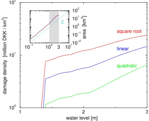
Fig. 7. Damage density and inundated area vs. water level. The
damage density, defined as damage per area, is plotted as a function of the water level for the non-coarse-grained mode with 4 nearest neighbours. We assume square root, linear, or quadratic building damage functions (from top), Eqs. (1), (3), and (4), see Fig. 2. The inset shows the inundated area as a function of the water level. The dotted line is a guide to the eye and follows a power-law with expo-nent 2. The grey area indicates the range of water levels shown in the main panel.
it appears already around 2 m and the remaining 2–3 m in-crease approximately linearly.
M. Boettle et al.: Influence of elevation model quality and small-scale damage functions 3333 increases approximately exponentially between 2.2 and 3 m,
which can be attributed to the corresponding damage func-tion (Fig. 6, lower set of curves).
5 Conclusions
We find that after a sudden jump, in any case the macro-scopic damage functions increase exponentially up to a cer-tain water level above which they change to a less steep in-crease, whereas the cross-over level depends on the assumed building damage function. Moreover, the range covered by the final damage functions obtained from the various modes of inundation determination differ by an approximately con-stant factor. In particular, we show that for large events the assumed building damage function dominates the final dam-age, while for small events the mode of coarse-graining has a dominating influence on the estimated damage.
Additional inundation methods could be obtained by vary-ing the way elevation heights are assigned to the buildvary-ings. As mentioned in Sect. 3, we defined the elevation of a build-ing as the height of the buildbuild-ing’s centre. Other Choices could be the minimum, maximum or average elevation of the terrain covered by the building. Since the available building information is a point dataset, these methods could not be ap-plied. However, we expect only an insignificant effect on the macroscopic damage, since the terrain in the case study area is rather flat and the buildings are small.
While the overall shape of the macroscopic damage func-tion likely depends on the local condifunc-tions of the considered area, it is plausible that the DEM and the building damage function should have a similar effect for moderate and heavy flood events, respectively, at other sites.
In general, we conclude that different regimes of a damage function have to be considered. With regard to low and mod-erate sea levels an accurate DEM is indispensable, since it provides information about whether low-lying properties are flooded or not. This can affect the total flood risk decisively because of the high frequency of such water levels. On the other hand, at higher flood levels, the building damage func-tion becomes more dominant than the quality of the DEM and although such events are very rare, the corresponding damages need careful estimations due to their catastrophic consequences.
Accordingly, our results suggest that depending on the flood height the DEM or the building damage function is more important.
Finally, it needs to be mentioned that climate change and sea level rise in many regions most likely lead to an increased frequency and magnitude of high water levels (Nicholls, 2004; Nicholls et al., 2007, and references therein). Accord-ing to our results, this might enter the regime where the build-ing damage functions become more important. This suggests that more research is needed to better estimate and determine building damage.
Acknowledgements. We would like to thank Jacob Arpe and the
municipality of Kalundborg for the provision of data and Lu´ıs Costa for fruitful discussions and comments. We appreciate financial support by the BaltCICA Project (part-financed by the EU Baltic Sea Region Programme 2007-2013).
Edited by: S. Tinti
Reviewed by: three anonymous referees
References
Apel, H., Aronica, G. T., Kreibich, H., and Thieken, A. H.: Flood risk analyses – how detailed do we need to be?, Nat. Hazards, 49, 79–98, 2009.
B¨uchele, B., Kreibich, H., Kron, A., Thieken, A., Ihringer, J., Oberle, P., Merz, B., and Nestmann, F.: Flood-risk mapping: contributions towards an enhanced assessment of extreme events and associated risks, Nat. Hazards Earth Syst. Sci., 6, 485–503, doi:10.5194/nhess-6-485-2006, 2006.
Dasgupta, S., Laplante, B., Meisner, C., Wheeler, D., and Yan, J.: The impact of sea level rise on developing countries: a compara-tive analysis, Clim. Change, 93, 379–388, 2008.
Dutta, D., Herath, S., and Musiake, K.: A mathematical model for flood loss estimation, J. Hydrol., 277, 24–49, 2003.
Gesch, D. B.: Analysis of Lidar Elevation Data for Improved Iden-tification and Delineation of Lands Vulnerable to Sea-Level Rise, J. Coastal Res., 53, 49–58, 2009.
Hallegatte, S., Ranger, N., Mestre, O., Dumas, P., Corfee-Morlot, J., Herweijer, C., and Muir Wood, R.: Assessing Climate Change Impacts, Sea Level Rise and Storm Surge Risk in Port Cities: A Case Study on Copenhagen, Clim. Change, 104, 113–137, 2011. Mazria, E. and Kershner, K.: Nation under siege: sea level rise at
our doorstep, The 2030 Research Center, 2007.
Merz, B. and Thieken, A. H.: Separating natural and epistemic un-certainty in flood frequency analysis, J. Hydrol., 309, 114–132, 2004.
Merz, B. and Thieken, A. H.: Flood risk curves and uncertainty bounds, Nat. Hazards, 51, 437–458, 2009.
Merz, B., Thieken, A. H., , and Bl¨oschl, G.: Uncertainty analysis for Flood Risk Estimation, in: International Conference on Flood Estimation, edited by: Spreafico, M. and Weingartner, R., CHR Report II-17, 577–585, 2002.
Merz, B., Kreibich, H., Thieken, A., and Schmidtke, R.: Estimation uncertainty of direct monetary flood damage to buildings, Nat. Hazards Earth Syst. Sci., 4, 153–163, doi:10.5194/nhess-4-153-2004, 2004.
Nascimento, N., Machado, M. L., Baptista, M., and Silva, A. D. P. E.: The assessment of damage caused by floods in the Brazil-ian context, Urban Water J., 4, 195–210, 2007.
Nicholls, R. J.: Coastal flooding and wetland loss in the 21st cen-tury: changes under the SRES climate and socio-economic sce-narios, Glob. Environmen. Change, 14, 69–86, 2004.
Poulter, B. and Halpin, P. N.: Raster modelling of coastal flooding from sea-level rise, Int. J. Geogr. Inf. Sci., 22, 167–182, 2008. Rowley, R. J., Kostelnick, J. C., Braaten, D., Li, X., and Meisel,
J.: Risk of Rising Sea Level to Population and Land Area, Eos Trans. AGU, 88, 105–116, 2007.