www.nat-hazards-earth-syst-sci.net/14/295/2014/ doi:10.5194/nhess-14-295-2014
© Author(s) 2014. CC Attribution 3.0 License.
Natural Hazards
and Earth System
Sciences
A data-based comparison of flood frequency analysis methods used
in France
K. Kochanek1, B. Renard2, P. Arnaud3, Y. Aubert3, M. Lang2, T. Cipriani2, and E. Sauquet2
1Institute of Geophysics, Polish Academy of Sciences, Ksi˛ecia Janusza 64, 01-452, Warsaw, Poland
2Irstea Lyon, UR HHLY Hydrology-Hydraulics, 5 rue de la Doua CS70077, 69626 Villeurbanne CEDEX, France 3Irstea Aix-En-Provence UR OHAX, 3275 Route de Cézanne, CS 40061, 13182 Aix-en-Provence CEDEX 5, France
Correspondence to: K. Kochanek ([email protected])
Received: 31 July 2013 – Published in Nat. Hazards Earth Syst. Sci. Discuss.: 6 September 2013 Revised: 8 January 2014 – Accepted: 10 January 2014 – Published: 20 February 2014
Abstract. Flood frequency analysis (FFA) aims at estimating
quantiles with large return periods for an extreme discharge variable. Many FFA implementations are used in operational practice in France. These implementations range from the estimation of a pre-specified distribution to continuous sim-ulation approaches using a rainfall simulator coupled with a rainfall–runoff model. This diversity of approaches raises questions regarding the limits of each implementation and calls for a nation-wide comparison of their predictive perfor-mances.
This paper presents the results of a national comparison of the main FFA implementations used in France. More accu-rately, eight implementations are considered, corresponding to the local, regional and local-regional estimation of Gum-bel and Generalized Extreme Value (GEV) distributions, as well as the local and regional versions of a continuous simu-lation approach. A data-based comparison framework is ap-plied to these eight competitors to evaluate their predictive performances in terms of reliability and stability, using daily flow data from more than 1000 gauging stations in France.
Results from this comparative exercise suggest that two implementations dominate their competitors in terms of pre-dictive performances, namely the local version of the con-tinuous simulation approach and the local-regional estima-tion of a GEV distribuestima-tion. More specific conclusions include the following: (i) the Gumbel distribution is not suitable for Mediterranean catchments, since this distribution demonstra-bly leads to an underestimation of flood quantiles; (ii) the lo-cal estimation of a GEV distribution is not recommended, be-cause the difficulty in estimating the shape parameter results in frequent predictive failures; (iii) all the purely regional
implementations evaluated in this study displayed a quite poor reliability, suggesting that prediction in completely un-gauged catchments remains a challenge.
1 Introduction
1.1 Diversity of flood frequency analysis approaches
1985, 1986; Hosking and Wallis, 1997), or combining local and regional information (e.g., Ribatet et al., 2006).
Many countries prepared and issued national FFA guide-lines to help practitioners in realizing their analyses with best practice methods, e.g., (Reed et al., 1999; Institution of Engineers Australia, 1987; Interagency Advisory Commit-tee on Water Data, 1982; Stewart et al., 2008). This is not the case in France, where no specific FFA implementation is officially recommended, let alone prescribed by regula-tion. While practitioner-oriented documents describing the main approaches to FFA have been published (Lang et al., 2007), an extensive comparison of the main FFA implemen-tations used in operational practice in France remains to be performed.
1.2 Challenges facing the evaluation and comparison of
FFA approaches
A large number of comparative studies of FFA implemen-tations have been reported in the research literature (e.g., Hosking et al., 1985; Gunasekara and Cunnane, 1992; Kroll and Stedinger, 1996; GREHYS, 1996; Ouarda et al., 2006; Meshgi and Khalili, 2009; Sankarasubramanian and Srini-vasan, 1999). The comparison framework varies from one study to another, and can be based on Monte Carlo simula-tions, statistical tests, graphical methods and so on. Bobee et al. (1993) therefore advocated “a systematic approach to comparing distributions used in flood frequency analysis”, which is still not agreed upon to our best knowledge.
In the context of the present paper, where distinct FFA families are to be compared, the comparison framework can hardly be based on Monte Carlo simulations. Indeed, this would require setting up a synthetic experiment to generate “true” data that can be used by all FFA implementations. En-suring a “fair” simulation setup that would not advantage a particular FFA implementation is feasible when similar im-plementations are considered (e.g., comparing several local estimation methods for a given distribution). However, it is more difficult when both local and regional estimation ap-proaches are considered: how to realistically simulate spa-tially dependent extremes on a river network? What is a alistic misspecification of the regression model used in re-gional approaches? Ensuring the fairness of the simulation setup is even more challenging if continuous simulation ap-proaches are considered (How to realistically simulate the non-linearity of the rainfall–runoff relationship? How to sim-ulate realistic structural errors for the rainfall simulator or the hydrologic model?).
An alternative to Monte Carlo comparisons is to imple-ment data-based predictive comparisons, where the estima-tions from all competing FFA implementaestima-tions are sim-ply compared with validation data (Gunasekara and Cun-nane, 1992; Interagency Advisory Committee on Water Data, 1982). Recently, Renard et al. (2013) proposed a data-based comparison framework that could be applied to any FFA
implementation. This framework complements (but not re-places) alternative comparison methods based, for instance, on Monte Carlo simulations. Most important, this framework enables the comparison of any FFA implementation belong-ing to each family presented in Sect. 1.1.
1.3 Objectives of the paper
In this paper we present the results of a nation-wide compar-ison of the predictive performances of FFA implementations in order to find the limits of each implementation and, if pos-sible, recommend the best FFA methodology for the French rivers. By best methodology we mean best performance of a particular implementation according to the indices described later in Sect. 2.3.
The paper is organized as follows. Section 2 presents the data and methods used in this paper, including the compet-ing FFA implementations (Sect. 2.2), a summary of the com-parison framework (Sect. 2.3) and the comcom-parison data set (Sect. 2.4). Section 3 describes the main results of the com-parison, and Sect. 4 further discusses them. Conclusions are drawn in Sect. 5.
2 Data and methods
2.1 Short description of the ExtraFlo project
By their nature and danger, the extreme floods cannot be ob-served often and thoroughly enough to collect the sample ad-equate for further statistical analysis. Instead, the probabilis-tic study of extreme values relies on the analysis of a lim-ited (in number and space) series of events in time, to infer a probabilistic behavior of a particular case which is then ex-trapolated to the whole population of floods. This procedure encounter certain difficulties:
– How to extrapolate excessively short time series, when
information is generally available on more or less re-cent events.
– How to set design values for the whole of the territory,
whereas the density of the measurement is inevitably limited owing to the spatial variability of rainfall and discharge data.
– How to update our knowledge of extreme events in a
non-stationary context.
some civil engineering structures (large dams, nuclear power plants) may require 103–104target return periods.
A particular emphasis was placed during the project on compiling reference data sets (long at-site time series and re-gional sets) to pinpoint the pros and cons of each approach with their sensitivity to the increasing information. As a re-sult of this work methods for estimating extreme values of floods were developed and improved. Moreover, the project placed a range of practical tools concerning the management of flood risk that can be estimated not only according to the hydrological characteristics of river basins but also on the basis of available information.
2.2 Competing teams: FFA implementations
Eight implementations that are frequently used in France are compared in this paper. Note that other approaches are also used in operational practice, in particular the SCHADEX semi-continuous simulation approach (Paquet et al., 2006) or the SPEED method (Cayla, 1995). However they could not be included in this comparative exercise because they could not be fully automated and were therefore not suitable for an application to thousands of sites (see Sect. 2.4). The eight competing implementations are split according to their esti-mation scale: purely local, purely regional or mixed local-regional.
2.2.1 The local league: using at-site runoff data only
The local league contains the following three implementa-tions:
1. Implementation LOC_GUM, corresponding to the es-timation of a two-parameter Gumbel distribution us-ing at-site annual maxima (see Sect. AA for details on the Gumbel distribution). A Bayesian estimation is performed, with flat priors (π(θ )∝1)for both the lo-cation and the scale parameters. Maximum-posterior values are used as parameter estimates.
2. Implementation LOC_GEV, corresponding to the es-timation of a three-parameter GEV distribution using at-site annual maxima (see Sect. AA for details on the GEV distribution). A Bayesian estimation is also per-formed, with flat priors (π(θ )∝1)for the location and the scale parameters, and a Gaussian prior with mean zero and standard deviation 0.25 for the shape param-eter.
3. Implementation LOC_SHY is the local version of the SHYREG method, a continuous simulation approach, coupling a rainfall generator with a rainfall–runoff model to estimate flood quantiles. A description of the various versions of SHYREG can be found in Arnaud and Lavabre (2002), Aubert (2013) and Organde et al. (2013).
For the first two implementations, the Gumbel and GEV distributions are chosen because they are the most widely used methods in hydrological projects in France (despite the fact that there is no prescribed distribution officially recommended for FFA in France). Moreover, preliminary analyses (not shown) indicated that they performed at least equally well as other distributions, including Log-Normal, Pearson III or Log-Pearson III distributions. The choice of the Bayesian estimation approach is made to facilitate the use of a unique estimation approach at local, regional and local-regional scales. Preliminary analyses (Kochanek et al., 2012; Renard et al., 2013) show that for a given record length, the impact of the estimation approach (e.g., Bayesian, maximum likelihood, moments, linear moments) is small compared to the choice of the parent distribution or the choice of the esti-mation scale (local, regional or local-regional). The analysis was carried out for the same record length (N )for the com-peting implementations (see Sect. 2.4 for details).
Regarding the third implementation, note that LOC_SHY uses a regionalized version of the rainfall generator, but is local with respect to discharge data in the sense that the rainfall–runoff model is estimated with local data. The re-gionalization of the rainfall generator is based on a data set comprising 2812 daily rain gauges with at least 20 years of data over the period 1977–2002 (Arnaud et al., 2008). Re-gionalization is performed for the three parameters of the rainfall generator, namely: the average number of storms, the average storm intensity and the average storm duration. Re-gionalized parameters are then available on a 1×1 km grid. The fact that these parameters represent averages over many storms (average number, intensity and duration) induces a much lesser sensitivity to sampling variability than more ex-treme characteristics (see Carreau et al., 2013).
2.2.2 The regional league: estimation in ungauged
catchments
The regional league contains the following three implemen-tations:
1. Implementation REG_GUM, corresponding to the re-gional estimation of a Gumbel distribution by means of regressions linking its parameters with catchment characteristics.
2. Implementation REG_GEV, corresponding to the re-gional estimation of a GEV distribution.
The third implementation REG_SHY uses the same re-gionalized rainfall generator as implementation LOC_SHY. However, unlike LOC_SHY, it uses a regionalized version of the rainfall–runoff model. The details of this regionalization procedure are given by Organde et al. (2013). In the current paper, the regionalization procedure is re-implemented based on the runoff data set used to compare the FFA implementa-tions (see Sect. 2.4). Since most of the runoff data set cov-ers the period 1969–2011, the regionalization of the rainfall– runoff model is based on a period that encompasses the pe-riod used for regionalizing the rainfall generator (1977–2002, see Sect. 2.2.1).
2.2.3 The local-regional league: combining at-site data
and regional information
The local-regional league contains the following two imple-mentations:
1. Implementation L+R_GUM, corresponding to the local-regional estimation of a Gumbel distribution, us-ing both local and regional information.
2. Implementation L+R_GEV, corresponding to the local-regional estimation of a GEV distribution. The combination of local and regional information is straightforward in the Bayesian context adopted here: re-gional estimates are used to specify a prior distribution, while local data are used to compute the likelihood function (see Sect. A2 for additional details).
2.3 Referees: stability and reliability indices
The evaluation criteria are based on performance indices quantifying the reliability and the stability of the FFA imple-mentations. A complete description of the motivation behind these performance indices is given in Renard et al. (2013). In this paper we therefore restrict ourselves to a short presenta-tion of these indices and their practical use to compare FFA implementations.
2.3.1 Reliability indices
The reliability indices aim to evaluate the agreement between the estimated distribution at sitei(whose cumulative distri-bution function, CDF, is notedFˆ(i))and validation observa-tionsdk(i)
k=1:n(i). Importantly, this requires splitting
avail-able data into calibration and validation subsamples. The decomposition adopted in this paper will be described in Sect. 2.4.
The first reliability index was used, e.g., by England et al. (2003) and Garavaglia et al. (2011), and corresponds to the CDF of the estimated distribution computed on the largest validation data. For a given sitei, it is computed as follows:
F F(i)= ˆF(i)(dmax(i) ). (1)
If the estimation is reliable (i.e.,Fˆ(i)=F(i), whereF(i) denotes the unknown true CDF), it can be shown (Renard et al., 2013) that FF(i)is a realization from a Beta distribu-tion with parameters (n(i); 1): FF(i)∼ Beta(n(i); 1), whose CDFFBetacan be written asFBeta(t )=tn
(i)
, 0≤t≤1. The
FF index focuses on the right tail of the estimated CDF by
using the largest element in the validation sample. The ade-quacy between FF(i)values observed over all validation sites and their theoretical Beta distributions under the reliability hypothesis will be assessed using graphical diagnostics and reliability scores that will be described in Secs. 2.3.3. and 2.3.4.
The second reliability index is based on the number of exceedances (within the validation sample) of an estimated
T-year quantileqˆT(i)(e.g., Interagency Advisory Committee on Water Data, 1982; Gunasekara and Cunnane, 1992; Gar-avaglia et al., 2011):
NT(i)=
n(i) X
k=1
1 ˆ
qT(i);+∞
dk(i), where 1A(x)=
1 ifx∈A
0 otherwise. (2)
Under the reliability assumptionqˆT(i)=qT(i),NT(i) is a realization from the binomial distribution:
NT(i)∼Binn(i),1/T
(Renard et al., 2013). TheNT index focuses on reliability for prescribed T-year quantiles. In this paper, we are going to analyzeNT=10andNT=100values for 10-year and 100-year floods, respectively.
2.3.2 Stability index
The stability of quantile estimates can be quantified by con-trasting the values obtained with two different calibration data sets c1 and c2. The decomposition into two calibra-tion subsamples adopted in this paper will be described in Sect. 2.4. We stress that the stability is only a secondary con-sideration compared to reliability: indeed, a FFA implemen-tation can be totally unreliable but perfectly stable. Conse-quently, stability is seen as an additional quality used to fur-ther discriminate FFA implementations that would have sim-ilar reliability.
The index SPANT (Garavaglia et al., 2011) used in this paper is a measure of the span of twoT-year quantiles esti-mated with distinct calibration data sets. For a given sitei, it is defined as follows:
SPAN(i)T =2
qˆ
(i) T (c1)− ˆq
(i) T (c2)
ˆ
qT(i)(c1)+ ˆqT(i)(c2)
. (3)
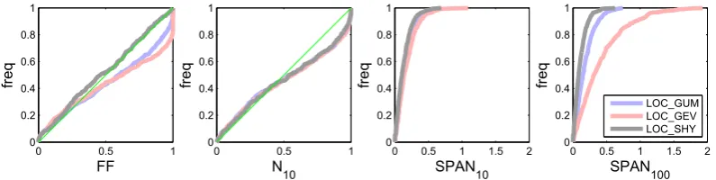
Fig. 1. Reliability (F F,N10) and stability (SPAN10, SPAN100) indices for local implementations.
2.3.3 Graphical representations
Reliability
Graphical representation of reliability is based on the com-parison between the calculated indices and their theoretical distribution under the reliability assumption. Note that for both reliability indices, this theoretical distribution depends on the number of validation observationsn(i), that may vary from site to site. To circumvent this problem, a probability-probability plot (pp-plot) representation is adopted: raw in-dices are transformed into probabilities by applying the CDF of their theoretical distribution under the reliability hy-pothesis. Under the reliability hypothesis, the probability-transformed values are then uniformly distributed between 0 and 1, regardless of the sample sizen(i). It is therefore pos-sible to plot the probability-transformed values for all sites against empirical frequencies, yielding reliability pp-plots as illustrated in Fig. 1. Curves closer to the diagonal correspond to more reliable FFA implementations.
Note that for theNT index, the theoretical binomial distri-bution is a discrete distridistri-bution. It is therefore necessary to randomize its probability-transformed values in order to en-sure that they are uniformly distributed. The randomization procedure is described in Renard et al. (2013).
Stability
The comparison of stability between competing FFA imple-mentations is based on comparing the distribution of SPAN(i)T over all sitesi=1:Nsites, as illustrated in Fig. 1. The FFA implementation whose SPANT distribution remains the clos-est to zero is the most stable.
2.3.4 Scores
The graphical representations can be further summarized into numerical scores that will provide a more synthetic view of the performances of FFA implementations over the various performance indices.
For reliability indices FF andNT, the score is based on the area between the diagonal line and the reliability curve, with a normalization ensuring that the score is varying be-tween 0 (low reliability) and 1 (perfect reliability). For any probability-transformed indexw, the score can be computed as
score=1−2·Area(curve,diagonal)=
=1− 2
Nsite+1 Nsite
X
i=1
w(i)−i−0.5
Nsite
. (4)
Analogically, a stability score can be derived based on the area between theyaxis and the SPANT curve, normalized to vary between 0 (low stability) and 1 (perfect stability):
score=1−0.5·Area(curve,yaxis)
=1− 1
2Nsite
Nsite
P
i=1
SPAN(i)T . (5)
2.4 Playground: daily runoff data set
2.4.1 Data set description
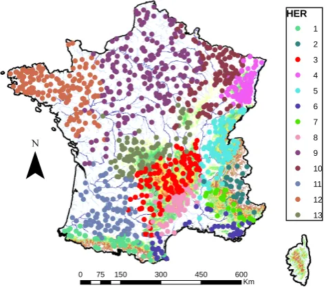
Daily runoff series from 1076 gauging stations located throughout France are used (see Fig. 2). Catchment sizes range from 10 to 2000 km2. All series have at least 20 years of data (20–39 years: 535 stations (49.7 %); 40–59 years: 476 stations (44.2 %); 60 years and more: 65 stations (6.1 %)). The quality-control procedures have been implemented to re-move stations with measurement problems or stations cor-responding to heavily regulated catchments. This data set is therefore an extension of the data set used by Renard et al. (2008), including updated series (until 2012) and many more stations.
!!! ! ! !!!!! ! !!!!!!!!!!!!!!!!! !! !!!! ! ! !!!! ! ! ! ! !! !! ! ! ! !! ! ! ! ! ! ! ! !!! ! ! ! !! ! ! ! ! ! ! ! ! ! ! !!!!!!!! ! !! ! ! !!!! ! ! !!!! !!!! ! ! ! !! ! ! ! ! ! ! ! ! !!! !!! ! ! ! ! !! ! ! !!! !!! ! !! ! ! !! ! ! !! ! ! ! ! ! ! ! ! ! ! ! ! ! ! ! ! !!!! ! !!!!!!! ! ! ! ! ! ! ! !!!!!!! ! ! ! ! ! ! !! !! !!! ! ! ! ! !!!! ! !!! !! ! !!!! !! ! ! !!! ! ! !! ! ! ! ! ! !! ! ! !! !!!! ! ! ! !! ! ! ! ! ! ! ! ! ! ! ! ! ! ! ! ! ! !!!! !!! ! ! !! !! ! !!! ! ! ! ! ! ! ! ! ! !! ! ! ! ! !! !! !! !! ! !! ! ! ! ! ! ! ! ! ! !! ! !! !! ! ! ! ! !! ! ! ! !! ! ! ! ! ! ! ! ! ! ! ! !!!!! !!! ! ! ! !!!!!!!!! !!!!!!!! ! ! ! ! !! !!!!!!!!!!!!!!!! ! ! ! !! !! !!!!! ! ! !! ! !! !! !!!! ! ! !!!! ! !!!!!!!!!! ! !! ! ! ! ! ! ! ! ! ! ! ! ! ! ! ! ! !! !!! ! ! ! ! ! ! !!! !!!!! ! ! !! ! ! ! ! ! ! ! ! ! ! ! !!! ! ! ! ! ! ! ! ! !!! ! ! !!! ! ! ! !!! ! ! ! ! ! !! !!!! ! !! ! ! ! !!! ! ! ! ! ! ! ! !! ! ! ! ! ! ! ! ! ! !!! ! ! ! ! ! ! ! ! ! ! !!!!! ! ! ! ! ! ! ! ! !! ! ! ! ! ! ! ! ! ! ! !! ! ! ! !!! ! ! ! ! ! ! !!!! ! ! ! ! !! ! ! ! ! !! ! ! ! !! ! ! ! ! ! ! ! !! ! !!!!!!! ! ! ! !! !!!! ! ! ! !!! !!!! !! !!! ! ! ! ! ! ! !! ! !!!!! ! ! ! ! ! ! ! !! ! ! ! ! ! ! ! ! !!!!!!! ! ! ! ! ! ! ! !! ! ! ! ! ! ! !! ! ! ! ! ! ! ! !! ! ! ! ! ! ! ! ! !!!!!! ! ! ! ! ! ! ! ! ! ! ! ! ! ! ! ! ! ! ! ! !!! ! ! ! ! ! ! ! ! ! ! ! ! ! ! ! ! ! ! !! ! ! ! ! ! ! ! ! ! ! ! !!!!!!!!!!! ! !! ! ! ! ! !!!! ! ! ! ! ! ! ! ! ! ! ! ! ! ! ! ! ! ! ! ! ! !!! ! !! !! ! ! ! ! ! ! ! ! ! ! ! ! ! ! ! !! ! ! ! ! ! ! ! ! ! !!! ! !!! ! ! ! !! ! ! ! ! !! ! ! !! !!!! !!!!! !! !! ! ! ! ! !!! ! ! ! !!!!!! ! !! !! ! ! ! ! ! ! ! ! ! ! !!!! !!!!!! ! ! ! ! ! ! ! !! ! ! ! ! ! ! ! ! ! ! !! !! ! ! !! ! ! ! !!!!! ! ! !!! ! ! ! ! !!!!!! !! !!!! ! ! !!! ! ! ! ! ! ! !! ! ! !!!! ! !! !! ! ! ! !!!!! ! ! ! ! ! ! ! ! !! ! !!!! ! ! ! ! !!!! !!! ! ! ! ! !! !! !! ! !! !! ! ! ! !!!!!!! !!!!!!!!!!!!! ! ! ! !!!!!!! !! ! ! !! ! ! ! ! !! ! !! !!!!!!!!!!!!!!!! ! !!!!!!! !!!!!!!! ! !
¯
0 75 150 300 450 600
Km HER ! 1 ! 2 ! 3 ! 4 ! 5 ! 6 ! 7 ! 8 ! 9 ! 10 ! 11 ! 12 ! 13
Fig. 2. Location of the gauging stations used in this study.
2.4.2 Reliability and stability decompositions
As explained in Sect. 2.3, the computation of reliability in-dices requires decomposition of all data set time series into calibration-validation subsamples. For stability the data sets are also divided into two subsamples: calibration data set no. 1 (c1)and calibration data set no. 2 (c2). These decompo-sitions are performed as follows: for reliability, the 593 se-ries with 20 to 40 years of data are used to calibrate regional implementations, or the regional part of local-regional im-plementations. The remaining 483 series (with more than 40 years of data) are further decomposed:
– 20 years are randomly chosen (independently on each
site) to calibrate the local implementations, or the local part of local-regional implementations.
– All remaining years (at least 20 years) are used as
val-idation data. Importantly, the valval-idation data are there-fore exactly the same for all implementations. For stability, two distinct types of decompositions are imple-mented:
– The type I decomposition focuses on stability with
re-spect to local data: for each of the 483 series with more than 40 years, 20 years are randomly assigned to thec1 subsample, and 20 other years are randomly assigned to thec2subsample. Obviously, purely regional imple-mentations are insensitive to this decomposition, since they do not use local data.
– The type II decomposition focuses on stability with
respect to regional data: the 593 series with 20 to
40 years of data are randomly split into two subsam-ples c1 and c2. Obviously, purely local implementa-tions are insensitive to this decomposition, since they do not use regional data.
3 Results
3.1 Comparison of quantile estimates
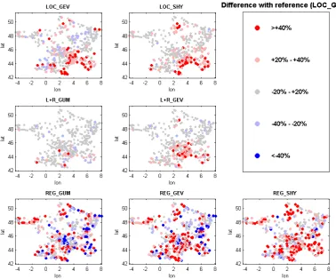
Before describing the comparison in terms of reliability and stability, it is of interest to assess how different the various competing implementations are. To this aim, Fig. 3 compares the 100-year flood estimated by each implementation with the one estimated by the implementation LOC_GUM, con-sidered as the reference in this figure.
Both local implementations LOC_GEV and LOC_SHY systematically yield larger quantiles in southeastern France (sometimes exceeding +40 %). Elsewhere in the country, smaller and larger quantiles are found with no clear spa-tial pattern for implementation LOC_GEV, while LOC_SHY quantiles tend to be systematically larger than LOC_GUM ones.
The local-regional implementation L+R_GUM generally yields small differences with the reference, suggesting that for a Gumbel distribution, local and local-regional estima-tions yield similar estimates. By contrast, the local-regional implementation L+R_GEV yields markedly higher quantiles in southeastern France.
All three regional implementations REG_GUM, REG_GEV and REG_SHY yield marked differences (both positive and negative) with the reference, but no distinctive spatial pattern can be observed. This suggests that the estimation scale (local or regional) has an important impact on quantile estimates.
3.2 Results for the local league
Figure 1 shows reliability and stability indices for the local implementations. Amongst them, LOC_SHY clearly outper-forms its two opponents (LOC_GUM and LOC_GEV): it is both more reliable (especially for extreme values, index FF) and more stable. The poor performance of the locally esti-mated GEV distribution is worth noting: it is markedly unre-liable and much less stable than other implementations (es-pecially for high quantiles). The behavior of the FF curves near the upper-right corner is noteworthy: it indicates that for about 20 % of the stations, a flood observed during the valida-tion period was deemed impossible by LOC_GEV (yielding
FF values equal to one). This is due to errors in estimating
Fig. 3. Relative differences between 0.99 quantiles.
Fig. 4. Reliability indices for regional implementations.
3.3 Results for the regional league
Figure 4 shows reliability indices for regional implemen-tations and shows that none of them reach an accept-able reliability. The continuous simulation implementation REG_SHY appears more reliable for index FF, but still yields unreliable predictions for the 10-year flood, as shown by indexN10. More detailed analyses (not shown here) sug-gest that the main reason for such poor performances is the difficulty in setting up a regression with catchments’ charac-teristics: the explanatory power of such regressions remains quite low and result in unreliable predictions at ungauged sites.
Note that we omitted the results in terms of stability for the regional implementations. Indeed, as noted in Sect. 2.3.2, stability is only a secondary consideration (compared with reliability) and is used only to discriminate implementations that would be comparably reliable. In this particular case, reliability is poor for all implementations (see Fig. 4), so we decided that stability was not worth considering (a stable but non-reliable implementation being worthless).
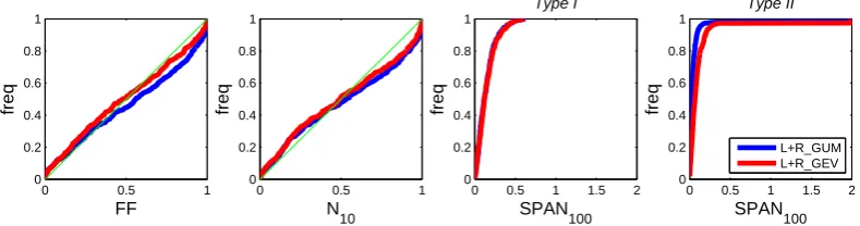
3.4 Results for the local-regional league
Figure 5 shows reliability and stability indices for the two local-regional implementations for Gumbel and GEV distri-butions. Both implementations yield similar results: the re-liability is acceptable and stabilities are similar. The use of a GEV distribution yields slightly more reliable predictions according to index FF, at the cost of a slightly lower stability with respect to regional information (type II). The differences between the Gumbel and GEV distributions will be further discussed in Sect. 3.5.
0 0.5 1 0
0.2 0.4 0.6 0.8 1
FF
fr
e
q
0 0.5 1
0 0.2 0.4 0.6 0.8 1
N 10
fr
e
q
0 0.5 1 1.5 2
0 0.2 0.4 0.6 0.8 1
fr
e
q
SPAN 100 Type I
0 0.5 1 1.5 2
0 0.2 0.4 0.6 0.8 1
fr
e
q
SPAN 100 Type II
L+R_GUM L+R_GEV
Fig. 5. Reliability (F F,N10) and stability (SPAN100– type I, SPAN100– type II) indices for local-regional implementations.
0 0.5 1
0 0.2 0.4 0.6 0.8 1
FF
fr
e
q
0 0.5 1
0 0.2 0.4 0.6 0.8 1
N 10
fr
e
q
0 0.5 1 1.5 2
0 0.2 0.4 0.6 0.8 1
fr
e
q
SPAN 100 Type I
0 0.5 1 1.5 2
0 0.2 0.4 0.6 0.8 1
fr
e
q
SPAN 100 Type II
LOC_GEV REG_GEV L+R_GEV
Fig. 6. Reliability (F F,N10) and stability (SPAN100– type I, SPAN100– type II) indices for local, regional and local-regional estimation of
a GEV distribution.
two opponents for both indices FF andN10. In terms of sta-bility, implementation L+R_GEV appears much more stable than both its purely local counterpart (type I stability) and its purely regional counterpart (Type II stability). These obser-vations confirm that the GEV distribution is a sensible can-didate for FFA, but that reliably estimating this distribution requires using both local and regional information.
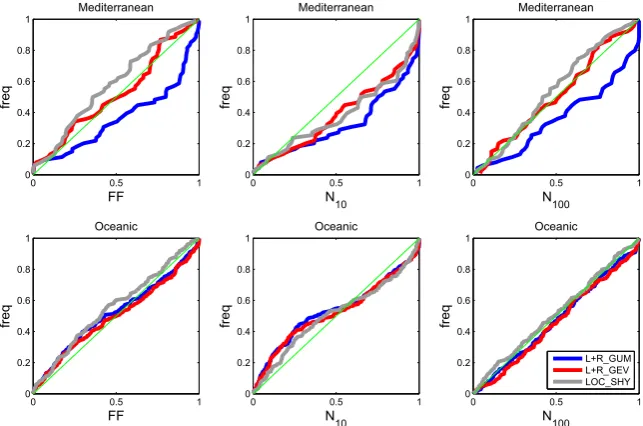
3.5 Stratification by region
The results were presented so far at the scale of the whole country. However, Sect. 3.1 suggested that the differences between some implementations followed specific regional patterns. Figure 7 therefore shows reliability indices for Mediterranean (top, corresponding to regions 6 and 8 in Fig. 2) and Oceanic (bottom, regions 9, 10, 12 and 13 in Fig. 2) catchments. For readability, only implementations LOC_SHY, L+R_GUM and L+R_GEV (which appear to be the most reliable ones) are presented.
For Mediterranean catchments, the use of a Gumbel distri-bution (L+R_GUM) consistently yields below-diagonal re-liability curves, denoting a tendency to underestimate quan-tiles. On the other hand, both implementations LOC_SHY and L+R_GEV yield acceptably similar reliability diagnos-tics. A tendency to slightly over-estimate large quantiles (in-dices FF andN100)might be suspected for LOC_SHY.
For Oceanic catchments, all three implementations yield similar results, suggesting that the evidence for rejecting the Gumbel distribution is weak in this region. We note however
that using a GEV distribution does not deteriorate reliability (as long as it is estimated with a local-regional approach), and might therefore be preferred to the Gumbel distribution for its larger flexibility.
Lastly, a note of caution is made for this figure regarding the indicesN10andN100. It might appear surprising at first sight that curves are closer from the diagonal forN100 than forN10. However, this does not suggest that estimates of the 100-year flood are more reliable than estimates of the 10-year flood. Indeed, while comparing implementations for a given reliability index makes complete sense, a comparison of reli-ability indices for a given implementation is not meaningful, because the power to detect non-reliability strongly varies from index to index. In this particular case, curves appear closer from the diagonal forN100mostly because detecting failures in the estimation of the 100-year flood is much more challenging than for the 10-year flood, given the available sample size.
3.6 Summary for all implementations
Fig. 7. Reliability indices for Mediterranean (top) and Oceanic (bottom) catchments.
0.60 0.70 0.80 0.90 1.00 FF
N10
N100
SPAN10 (I)
SPAN100 (I) SPAN1000 (I)
SPAN10 (II) SPAN100 (II)
SPAN1000 (II)
LOC_GUM LOC_GEV REG_GUM REG_GEV L+R_GUM L+R_GEV LOC_SHY REG_SHY
Fig. 8. Summary of reliability and stability scores for all imple-mentations.
catchments. Note that implementation L+R_GUM is not considered as a finalist because, despite its excellent sta-bility, it is systematically less reliable than LOC_SHY or L+R_GEV, and has been shown to be inadequate in the Mediterranean region (Sect. 3.5).
4 Discussion
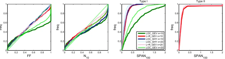
4.1 Results for different local sample sizes
The results presented in this paper are conditional on the par-ticular decompositions that were set up for stability and relia-bility assessments, and more precisely, on the sample size of 20 years for local data. One may therefore question whether the main findings of this study would still hold with different sample sizes.
Figure 9 indicates that the performances of the local-regional implementation L+R_GEV and of LOC_SHY are not very sensitive to the local sample size. On the other hand,
the performances of the local implementation LOC_GEV strongly deteriorate when the local sample size decreases. This indicates that the general conclusions summarized in Sect. 3.6 hold even more markedly with short samples.
Unfortunately, evaluating how performances evolve with larger samples is more challenging within this data-based comparison framework: indeed, the available series are not long enough to implement insightful calibration-validation decompositions with, e.g., 40 years used for calibration. The performance of local implementations is likely to improve with largest calibration samples. However, whether or not this would suffice to bridge the gap with the best imple-mentations (L+R_GEV and LOC_SHY) remains to be seen. Monte Carlo experiments suggest that estimation errors can remain quite large even with “long” series of 40–50 years (not shown). This suggests that the benefit of complementing local data with either regional information (L+R_GEV) or information on the rainfall–runoff relationship (LOC_SHY), as advocated by Merz and Blöschl (2008a, b) and Viglione et al. (2013), may well remain significant with larger samples.
4.2 Comparison with literature results
Fig. 9. Reliability (F F,N10) and stability (SPAN100– type I, SPAN100– type II) indices for three implementations, using 10 or 20 years of
local data for calibration.
The main original results brought by this study are related to the comparison between distinct families of FFA imple-mentations, including two distinct paradigms (estimation of a pre-specified distribution vs. continuous simulation) and sev-eral estimation scales (local, regional, local-regional). Such between-family comparisons are much more scarce in the lit-erature. As far as we know, there have been no studies that reported Monte Carlo investigations to compare such distinct families, which is most probably due to the difficulty in set-ting up a fair Monte Carlo experiment, as explained in the introduction. Some authors compared the estimates arising from distinct families (e.g., Neppel et al., 2007), but they re-stricted the description to the differences between families, as opposed to ranking them according to their predictive per-formances. The evaluation carried out in this paper moves one step further by assessing and comparing predictive per-formances, which is necessarily a data-based exercise. For instance, the fact that the continuous simulation implemen-tation LOC_SHY yields reliable predictions could not have been convincingly demonstrated using Monte Carlo simula-tions only (see discussion in Sect. 2.1).
Another result worth mentioning is the demonstrated inad-equacy of the Gumbel distribution in Mediterranean catch-ments. The choice between a light-tailed Gumbel distribu-tion and a heavy-tailed GEV distribudistribu-tion has been the subject of important debates in the literature: recently, global analy-ses were performed by Papalexiou and Koutsoyiannis (2013) and Serinaldi and Kilsby (2014) to assess this issue for ex-treme daily precipitations. Overall, at-site estimation sug-gests a preferentially heavy-tailed behavior of extreme rain-fall at the global scale. The approach proposed in this pa-per might complement these analyses by evaluating whether using a light-tailed distribution leads to some demonstrable predictive failure in some regions of the world. Moreover, a joint assessment of the extremal behavior of both precipita-tion and streamflow at the global scale would also be of great interest.
4.3 Limitations of the comparison framework
While the comparison framework yielded valuable insights on the relative merits of distinct implementations, it is still
affected by several limitations that are discussed here. Firstly, the ability to detect predictive failures for large quantiles is restricted by the length of available data. With the typical sample sizes (40–100 years), demonstrating a prediction fail-ure for a 1000- or 10 000-year quantile (which are of inter-est for risky structures such as dams or nuclear plants, for instance) is affected by huge uncertainty (see also Klemeš, 2000 and Serinaldi, 2013). In this paper, we focus on the 10 to 100-year range. We do not consider floods of larger re-turn period (i.e.,>100 years), since the data-based compar-ison framework is not powerful enough to draw conclusions for such large quantiles. It is therefore unclear whether the good performances of some implementations (LOC_SHY and L+R_GEV), as evaluated with limited sample sizes, still hold for extreme quantiles. On the other hand, the implemen-tations showing poor performances have no reason to become highly capable when extrapolated to extreme quantiles, and can, therefore, be discarded.
A second limitation is related to the graphical nature of the comparison between implementations. It would be benefi-cial to implement a more quantitative comparison, e.g., based on hypothesis testing. For instance, it would be tempting to add significance limits around the diagonal in reliability plots (e.g., Fig. 4), as suggested by, e.g., Laio and Tamea (2007) based on a Kolmogorov–Smirnov test. Unfortunately, this cannot be done here because the test assumes independent data, but the values taken by the reliability indices are not fully independent from site to site (due to the spatial depen-dence existing between series from nearby sites).
Another limitation is that the comparison framework only produces global performance diagnostics, computed over a large number of sites. As a consequence, one should keep in mind that an implementation with excellent global perfor-mance may still fail on one or a few particular sites, with-out such isolated failures being detected by the global per-formance diagnostics.
which are also of primary interest in engineering practice (e.g., flood peak estimation for flood design).
5 Conclusions
The objective of this paper was to report the results of a national comparison of the main FFA approaches used in France. This comparison was performed within a data-based framework, which enabled a direct assessment of the predic-tive performances of candidate FFA approaches. The main conclusions that can be drawn from the work can be summa-rized in the following points:
1. Two approaches, namely the local version of SHYREG and the local-regional estimation of a GEV distribution, seem to provide generally satisfactory re-sults in terms of reliability and stability. The differ-ences between the quantiles estimated by these two ap-proaches are technically moderate.
2. In general, a local-regional estimation approach yields at least as good performances as its purely local or re-gional counterpart, and in some cases, it even clearly outperforms both of them.
3. In the oceanic-influenced catchments, the use of a Gumbel distribution seems acceptable. Local estimates yield relatively good performance indices. However the use of either the Gumbel or the GEV distribution within the mixed local-regional estimation approach results in similar or slightly improved reliability and stability indices.
4. In the Mediterranean area, we would not recommend using the Gumbel distribution, because it demonstra-bly underestimates quantiles. However, the local es-timation of a GEV distribution is not recommended either, because the difficulty in estimating the shape parameter results in a clear lack of reliability. There-fore we recommend using LOC_SHY or local-regional mixed procedure for estimating the GEV-based quan-tiles in this area.
5. Estimation of flood quantiles in ungauged catchments remains a genuine challenge: all competing regional approaches evaluated in this work lead to a quite low reliability.
These main results suggest several avenues for future work. First, improving the purely regional FFA implementations appears to be a priority, given their quite low reliability. This requires improving the regression linking model parameters with catchment descriptors. A first possibility to achieve this improvement may be to include other descriptors. Alternative strategies include moving from fixed regions to a region-of-influence approach (e.g., Burn, 1990; Haddad and Rahman,
2012), or using specialized geostatistical methods to transfer information along the hydrologic network (e.g., Gottschalk, 1993; Sauquet, 2006; Skøien et al., 2006; Laaha et al., 2014). In addition, combining several implementations may also yield further improvement. In particular, combining the best-performing implementations LOC_SHY and L+R_GEV would make use of both regional and rainfall information to complement local discharge data. This would correspond to the spatial and causal expansion of information recently ad-vocated by Merz and Blöschl (2008a, b), and implemented in a Bayesian framework by Viglione et al. (2013).
Appendix A
Local implementations
The PDF and CDF of the Gumbel distribution are
f (x)=1
λexp − x−µ
λ −exp − x−µ
λ
F (x)=exp−exp −x−µ
λ
λ >0,
(A1)
whereµandλare the location and the scale parameters. The PDF and CDF of the GEV distribution are
f (x)=1
λ
1−ξ(x−µ)
λ
1ξ−1
exp
−1−ξ(x−µ)
λ
1ξ
F (x)=exp
−1−ξ(x−µ)
λ
1ξ
λ >0, ξ6=0,1−ξ(x−µ)
λ >0,
(A2)
whereµ,λandξ are the location, scale and shape parame-ters.
Note that three families of distributions can be obtained depending on the value of the shape distribution: the Frechet family (ξ <0, left-bounded distribution), the Weibull family (ξ >0, right-bounded distribution) and the Gumbel family (ξ→0, unbounded distribution).
A1 Regional implementations
The regional estimation of Gumbel and GEV distributions uses a regression to link locally estimated parameters with catchment characteristics. Letθidenote the locally estimated location or scale parameter at sitei, σi denote its estima-tion standard deviaestima-tion (i.e., the posterior standard deviaestima-tion in this Bayesian context), and xi(1), . . . , x(Ncov)
i denote a set of Ncov catchment characteristics used as covariates. The regression model for location and scale parameters can be written as follows:
log(θi)=β0+ Ncov
X
j=1
βjxi(j )+εi, εi∼N (0,
q
σ2
0 10 20 -0.5
0 0.5
HER 1
station
ξ
0 5 -0.5
0 0.5
HER 2
station
ξ
0 50 -0.5
0 0.5
HER 3
station
ξ
0 20 40 -0.5
0 0.5
HER 4
station
ξ
0 20 40 -0.5
0 0.5
HER 5
station
ξ
0 20 -0.5
0 0.5
HER 6
station
ξ
0 5 10 -0.5
0 0.5
HER 7
station
ξ
0 10 20 -0.5
0 0.5
HER 8
station
ξ
0 50 100 -0.5
0 0.5
HER 9
station
ξ
0 50 -0.5
0 0.5
HER 10
station
ξ
0 20 40 -0.5
0 0.5
HER 11
station
ξ
0 50 -0.5
0 0.5
HER 12
station
ξ
0 20 -0.5
0 0.5
HER 13
station
ξ
Local estimations (95% intervals)
Regional estimation (95% interval)
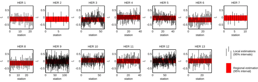
Fig. A1. Comparison of local and regional estimates of the shape parameter of a GEV distribution in each of the 13 hydroecoregions (HER).
relationship with catchment characteristics could be found, a constant regression is specified as follows:
ξi=β0+εi, εi∼N (0,
q
σ2
ε +σi2). (A4)
Catchment characteristics are selected following Cipri-ani et al. (2012): (i) catchment area; (ii) mean elevation; (iii) mean 10-year rainfall (as given by Benichou and Le Breton, 1987); (iv) mean IDPR index (Index of Develop-ment and Persistence of the River networks (Mardhel et al., 2004), used as a proxy for the infiltration capacity). More-over, regressions are estimated separately for each of the hy-droecoregions shown in Fig. 2. Note that all four predictors are systematically used for all regions. A Bayesian estima-tion is used (with flat priors on β0, . . . , βNcov,log(σε)
). Note that Eq. (A4) effectively assumes that the shape pa-rameter remains constant in each of the 13 hydroecoregions shown in Fig. 2. Empirical investigations suggest that this as-sumption is reasonable. As an illustration, Fig. A1 compares the local and regional estimates of the shape parameter: given estimation uncertainties, there is no strong evidence to reject the hypothesis of a constant shape parameter.
A2 Local-regional implementations
In local-regional implementations, a regional estimation is first applied to derive a prior distribution. At a given sitei,
the prior distribution of the location parameter is given by log(µi)∼N (µˆi,σˆε(µ)).µˆi is computed by applying the re-gression in Eq. (A3), i.e.,µˆi=exp βˆ0+
Ncov
P
j=1
ˆ
βjx (j ) i
!
, and
ˆ
σε(µ)is the estimated standard deviation of regression errors. Similarly, priors for the scale and shape parameters are given by
– Scale: log(λi)∼N (λˆi,σˆε(λ))
– GEV-only Shape:ξi ∼N (ξˆi,σˆε(ξ ))
At-site data are then used to compute the likelihood, and the posterior distribution therefore combines local and re-gional information.
Acknowledgements. This work was funded by the French Research Agency (ANR-08-RISKNAT-003) through the project ExtraFlo 2009-2013 (http://extraflo.irstea.fr/) and the FloodFreq COST Action ES0901 “European procedures for flood frequency estima-tion”. We thank Francesco Serinaldi and John England for their very helpful comments and Claire Lauvernet for her invaluable technical assistance.
Edited by: T. Kjeldsen
Reviewed by: F. Serinaldi and J. England
References
Arnaud, P. and Lavabre, J.: Using a stochastic model for generating hourly hyetographs to study extreme rainfalls, Hydrol. Sci. J., 44, 433–446, 1999.
Arnaud, P. and Lavabre, J.: Coupled rainfall model and discharge model for flood frequency estimation, Water Resour. Res., 38, 11-1–11-11, doi:10.1029/2001WR000474, 2002.
Arnaud, P., Lavabre, J., Sol, B., and Desouches, C.: Regionalization of an hourly rainfall-generating model over metropolitan France for flood hazard estimation, Hydrol. Sci. J., 53, 34–47, 2008. Aubert, Y.: Estimation des valeurs extrêmes de débit par la méthode
Shyreg: Réflexions sur l’équifinalité dans la modélisation de la transformation pluie en débit, Pierre and Marie Curie University, Irstea Aix-en-Provence, 316 pp., 2013.
Benichou, P. and Le Breton, O.: Prise en compte de la topographie pour la cartographie des champs pluviométriques statistiques, La Météorologie, 7, 23–34, 1987.
Bobee, B., Cavadias, G., Ashkar, F., Bernier, J., and Rasmussen, P.: Towards a Systematic-Approach to Comparing Distributions Used in Flood Frequency-Analysis, J. Hydrol., 142, 121–136, 1993.
Carreau, J., Neppel, L., Arnaud, P. and Cantet, P.: Extreme rainfall analysis at ungauged sites in the South of France: comparison of three approaches, Journal de la Société Française de Statistique, 154, 119–138, 2013.
Cayla, O.: Probability calculation of design floods and inflows – SPEED, Waterpower 1995, San Francisco, USA, 1995. Cipriani, T., Toilliez, T., and Sauquet, E.: Estimating 10 year return
period peak flows and flood durations at ungauged locations in France, La houille blanche, 2012.
England, J. F., Jarrett, R. D., and Salas, J. D.: Data-based compar-isons of moments estimators using historical and paleoflood data, J. Hydrol., 278, 172–196, 2003.
Garavaglia, F., Lang, M., Paquet, E., Gailhard, J., Garçon, R., and Renard, B.: Reliability and robustness of rainfall compound dis-tribution model based on weather pattern sub-sampling, Hydrol. Earth Syst. Sci., 15, 519–532, doi:10.5194/hess-15-519-2011, 2011.
Gottschalk, L: Correlation and covariance of runoff, Stochastic Hy-drology and Hydraulics, 7, 85–101, 1993.
GREHYS: Inter-comparaison of regional flood frequency proce-dures for Canadian rivers., J. Hydrol., 186, 85–103, 1996. Gunasekara, T. A. G. and Cunnane, C.: Split Sampling Technique
for Selecting a Flood Frequency-Analysis Procedure, J. Hydrol., 130, 189–200, 1992.
Haddad, K. and Rahman, A: Regional flood frequency analysis in eastern Australia: Bayesian GLS regression-based methods within fixed region and ROI framework – Quantile Regression vs. Parameter Regression Technique, J. Hydrol., 430–431, 142– 161, doi:10.1016/j.jhydrol.2012.02.012, 2012.
Hosking, J. R. M. and Wallis, J. R.: Regional Frequency Analysis: an approach based on L-Moments, Cambridge University Press, Cambridge, UK, 226 pp., 1997.
Hosking, J. R. M., Wallis, J. R., and Wood, E. F.: An appraisal of the regional flood frequency procedure in the UK flood studies report, Hydrol. Sci. J., 30, 85–109, 1985.
Institution of Engineers Australia: Australian Rainfall and Runoff, edited by: Pilgrim, D. H., Engineers Australia, 1987.
Interagency Advisory Committee on Water Data: Guidelines for de-termining flood-flow frequency: Bulletin 17B of the Hydrology Subcommittee, edited by: Coordination, O. o. W. D., US Geolog-ical Survey, Reston, Va., 1982.
Klemeš, V.: Tall tales about tails of hydrological distributions, II, J. Hydrol. Eng., 5, 232–239, doi:10.1061/(ASCE)1084-0699(2000)5:3(232), 2000.
Kochanek, K., Renard, B., Lang, M., and Arnaud, P.: Comparison of several at-site flood frequency models on a large set of French discharge series, The 2nd European Conference on FLOODrisk Management. Science Policy and Practice: Closing the Gap, Rot-terdam, the Netherlands, 2012.
Kroll, C. N. and Stedinger, J. R.: Estimation of moments and quan-tiles using censored data, Water Resour. Res., 32, 1005–1012, 1996.
Kuczera, G.: Comprehensive at-site flood frequency analysis using Monte Carlo Bayesian inference, Water Resour. Res., 35, 1551– 1557, 1999.
Laaha, G., Skøien, J. O., and Blöschl, G.: Spatial prediction on river networks: comparison of top-kriging with regional regression, Hydrol. Process., 28, 315–324, doi:10.1002/hyp.9578, 2014.
Laio, F. and Tamea, S.: Verification tools for probabilistic forecasts of continuous hydrological variables, Hydrol. Earth Syst. Sci., 11, 1267–1277, doi:10.5194/hess-11-1267-2007, 2007. Lang, M., Lavabre, J., Sauquet, E., and Renard, B.: Guide
méthodologique pour l’estimation de la crue centennale dans le cadre des plans de prévention des risques d’inondation, edited by: Quae, E., Editions Quae, 134 pp., 2007.
Mardhel, V., Frantar, P., Uhan, J., and Mio, A.: Index of develop-ment and persistence of the river networks as a component of regional groundwater vulnerability assessment in Slovenia, Int. Conf. groundwater vulnerability assessment and mapping, Us-tron, Poland, 2004.
Martins, E. S. and Stedinger, J. R.: Generalized maximum-likelihood generalized extreme-value quantile estimators for hy-drologic data, Water Resour. Res., 36, 737–744, 2000.
Merz, R. and Blöschl, G.: Flood frequency hydrology: 1. Temporal, spatial, and causal expansion of information, Water Resour. Res., 44, W08432, doi:10.1029/2007WR006744, 2008a.
Merz, R. and Blöschl, G.: Flood frequency hydrology: 2. Combining data evidence,Water Resour. Res., 44, W08433, doi:10.1029/2007WR006745, 2008b.
Meshgi, A. and Khalili, D.: Comprehensive evaluation of regional flood frequency analysis by L- and LH-moments. II. Develop-ment of LH-moDevelop-ments parameters for the generalized Pareto and generalized logistic distributions, Stoch. Environ. Res. Risk As-sess., 23, 137–152, 2009.
Neppel, L., Arnaud, P., and Lavabre, J.: Extreme rainfall mapping: Comparison between two approaches in the Mediterranean area, C. R. Geosci., 339, 820–830, doi:10.1016/j.crte.2007.09.013, 2007.
Organde, D., Arnaud, P., Fine, J.-A., Fouchier, C., Folton, N., and Lavabre, J.: Régionalisation d’une méthode de prédétermina-tion de crue sur l’ensemble du territoire français : la méthode SHYREG, Revue des sciences de l’eau, J. Water Sci., 26, 65–78, doi:10.7202/1014920ar, 2013.
Ouarda, T., Cunderlik, J. M., St-Hilaire, A., Barbet, M., Bruneau, P., and Bobee, B.: Data-based comparison of seasonality-based re-gional flood frequency methods, J. Hydrol., 330, 329–339, 2006. Papalexiou, S. M. and Koutsoyiannis, D.: Battle of extreme value distributions: A global survey on extreme daily rainfall, Water Resour. Res., 49, doi:10.1029/2012WR012557, 2013.
Paquet, E., Gailhard, J., and Garcon, R.: Evolution de la méth-ode du gradex: approche par type de temps et modélisation hy-drologique, La houille blanche, 5, 80–90, 2006.
Reed, D. W., Faulkner, D. S., Robson, A. J., Houghton-Carr, H., and Bayliss, A. C.: Flood Estimation Handbook, edited by: Institute of Hydrology, Wallingford, 1999.
Renard, B., Lang, M., Bois, P., Dupeyrat, A., Mestre, O., Niel, H., Sauquet, E., Prudhomme, C., Parey, S., Paquet, E., Neppel, L., and Gailhard, J.: Regional methods for trend detection: Assess-ing field significance and regional consistency, Water Resour. Res., 44, W08419, doi:10.1029/2007WR006268, 2008. Renard, B., Kochanek, K., Lang, M., Garavaglia, F., Paquet, E.,
Ribatet, M., Sauquet, E., Gresillon, J. M., and Ouarda, T. B. M. J.: A regional Bayesian POT model for flood frequency analysis, Stoch. Environ. Res. Risk Assess., 21, 327–339, 2006.
Sankarasubramanian, A. and Srinivasan, K.: Investigation and com-parison of sampling properties of L-moments and conventional moments, J. Hydrol., 218, 13–34, 1999.
Sauquet, E: Mapping mean annual river discharges: Geostatisti-cal developments for incorporating river network dependencies, J. Hydrol., 331, 300–314, doi:10.1016/j.jhydrol.2006.05.018, 2006.
Serinaldi, F.: An uncertain journey around the tails of multivariate hydrological distributions, Water Resour. Res., 49, 6527–6547, doi:10.1002/wrcr.20531, 2013.
Serinaldi, F. and Kilsby, C. G.: Rainfall extremes: Towards recon-ciliation after the battle of distributions, Water Resour. Res., 50, doi:10.1002/2013WR014211, 2014.
Skøien, J. O., Merz, R., and Blöschl, G.: Top-kriging – geostatis-tics on stream networks, Hydrol. Earth Syst. Sci., 10, 277–287, doi:10.5194/hess-10-277-2006, 2006.
Stedinger, J. R. and Tasker, G. D.: Regional hydrologic analysis: 1. Ordinary, weighted and generalized least squares compared, Water Resources Research, 21, 1421–1432 [Correction, Water Resour. Res., 1422, 1844, 1986.], 1985.
Stedinger, J. R. and Tasker, G. D.: Regional hydrologic analysis: 2. Model-error estimators, estimation of sigma and log-Pearson type 3 distributions, Water Resour. Res., 22, 1487–1499, 1986. Stewart, E. J., Kjeldsen, T. R., Jones, D. A., and Morris, D. G.: The
flood estimation handbook and UK practice:past, present and fu-ture, in: Flood Risk Management: Research and Practice, edited by: Samuels, P., Huntington, S., Allsop, W., and Harrop, J., CRC Press, 179, 2008.
Viglione, A., Merz, R., Salinas, J. L., and Blöschl, G.: Flood fre-quency hydrology: 3. A Bayesian analysis, Water Resour. Res., 49, 675–692, doi:10.1029/2011WR010782, 2013.