1
Performance Analysis of Reliability Growth
Models using Supervised Learning Techniques
Y Vamsidhar, P Samba Siva Raju, T Ravi Kumar
Abstract— Software reliability is one of a number of aspects of computer software which can be taken into consideration when determining the quality of the software. Building good reliability models is one of the key problems in the field of software reliability. A good software reliability model should give good predictions of future failure behavior, compute useful quantities and be widely applicable. Software Reliability Growth Models (SRGMs) are very important for estimating and predicting software reliability. An ideal SRGM should provide consistently accurate reliability estimation and prediction across different projects. However, that there is no single such model which can obtain accurate results for different cases. The reason is that the performance of SRGMs highly depends on the assumptions on the failure behavior and the application data-sets. In other words, many models may be shown to perform well with one failure data-set, but bad with the other data-set.
Thus, combining some individual SRGMs than single model is helpful to obtain a more accurate estimation and prediction. SRGM parameters are estimated using the least square estimation (LSE) or Maximum Likelihood Estimation (MLE). Several combinational methods of SRGMs have been proposed to improve the reliability estimation and prediction accuracy. The AdaBoosting algorithm is one of the most popular machine learning algorithms. An AdaBoosting based Combinational Model (ACM) is used to combine the several models. The key idea of this approach is that we select several SRGMs as the weak predictors and use an AdaBoosting algorithm to determine the weights of these models for obtaining the final linear combinational model. In this paper, the Fitness and Prediction of various Software Reliability Growth Models (SRGMs) can be compared with AdaBoosting based Combinational Model (ACM) with the help of Maximum likelihood estimation to estimate the model parameters.
Index Terms— Software Reliability, Software Reliability Growth Models (SRGMs), AdaBoosting Algorithm, Least Square Estimation,
Maximum Likelihood Estimation.
—————————— ——————————
1
INTRODUCTIONOFTWARE Reliability Engineering is defined as quantitative study of the operational behavior of
software-based systems with respect to user requirements
concerning reliability. The demand for software systems has recently increased very rapidly. The reliability of software
systems has become a critical issue in the software systems
industry. With the 90’s of the previous century, computer
software systems have become the major source of reported failures in many systems. Software is considered reliable if
anyone can depend on it and use it in critical systems. The
importance of software reliability will increase in the years to come, specifically in the fields of aerospace industry, satellites,
and medicine applications. The process of software reliability
starts with software testing and gathering of test results, after
that, the phase of building a reliability model.
In general, the concept of reliability can be defined as
“the probability that a system will perform its intended
function during a period of running time without any failure”. IEEE defines software reliability as “the probability of
failure-free software operations for a specified period of time in a
specified environment”. In other words, software reliability
can be viewed as the analysis of its failures, their causes and
effects. Software reliability is a key characteristic of product quality. Most often, specific criteria and performance
measures are placed into reliability analysis, and if the
performance is below a certain level, failure occurred. Mathematically, the reliability function R(t) is the probability
that a system will be successfully operating without failure in
the interval from time 0 to time t [1],
R(t) = P(T>t), where t >=0
T is a random variable representing the failure time or
time-to-failure (i.e. the expected value of the lifetime before a
failure occurs). R(t) is the probability that the system's lifetime is larger than (t), the probability that the system will survive
beyond time t, or the probability that the system will fail after
time t. From above Equation, we can conclude that failure
probability F(t), unreliability function of T is:
F(t) = 1 – R(t) = P(T<=t)
If the time-to-failure random variable T has a density function
f(t), then the reliability can be measured as following
R(t) = f(x) dx
Where f(x) represents the density function for the random
variable T. Consequently, the three functions R(t), F(t) and f(t) are closely related to one another .
S
————————————————
Y Vamsidhar is working as Assoc. Professor & HOD, CSE Dept., Swarnandhra College of Engg. & Technology, Narsapur, W.G.Dist. (A.P), India, PH-00919849523241. E-mail: [email protected]
P Samba Siva Raju is working as Asst. Professor, CSE Dept., VISIT Engg. College, Tadepalligudem, W.G.Dist. (A.P), India, PH-00919951722365. E-mail: [email protected]
©2012
2
2
S
UPERVISEDL
EARNINGT
ECHNIQUES2.1 Bootstrap
The Bootstrap procedure is a general purpose sample-based
statistical method which consists of drawing randomly with
replacement from a set of data points. It has the purpose of assessing the statistical accuracy of some estimate, say S(Z),
over a training set Z = {z1, z2, . . . , zN}, with zi = (xi, yi). To
check the accuracy, the measure is applied over the B sampled
versions of the training set. The Bootstrap algorithm[10] is as follows:
Bootstrap Algorithm
Input:
Training set Z={z1,z2,…,zN}, with zi=(xi,yi).
B, number of sampled versions of the training set.
Output:
S(Z), statistical estimate and its accuracy. Step 1:
for n=1 to B
a) Draw, with replacement, L < N samples from the training set Z, obtaining the nth sample Z*n.
b) For each sample Z*n, estimate a statistic S(Z*n).
Step 2:
Produce the bootstrap estimate S(Z), using S(Z*n) with n = {1, .
. . ,B}. Step 3:
Compute the accuracy of the estimate, using the variance or
some other criterion.
We start with the training set Z, obtaining several versions Z*n
(bootstrap samples). For each sampled version, we compute the desired statistical measure S(Z*n).
2.2 Bagging
The Bagging technique[10] consists of Bootstrap aggregation.
Let us consider a training set Z ={z1, z2, . . . , zN}, with zi = (xi,
yi) for which we intend to fit a regression model, obtaining a
prediction f(x) at input x. Bagging averages this prediction over a collection of bootstrap samples, thereby reducing its
variance.
For classification purposes, the Bagging algorithm is as follows.
Bagging Algorithm for Classification
Input:
Z = {z1, z2, . . . , zN}, with zi = (xi, yi) as training set.
B, number of sampled versions of the training set.
Output:
H(x), a classifier suited for the training set.
Step 1: for n=1 to B
a) Draw, with replacement, L < N samples from the training
set Z, obtaining the nth sample Z*n. b) For each sample Z*n, learn classifier Hn.
Step 2:
Produce the final classifier as a vote of Hn with n = {1, . . . ,B}
H(x)= sign (ΣB
n=1 Hn(x))
As compared to the process of learning a classifier in a
conventional way, that is, strictly from the training set, the Bagging approach increases classifier stability and reduces
variance.
2.3 Boosting
The Boosting[10] procedure is similar to Bootstrap and
Bagging. The first was proposed in 1989 by Schapire and is as
follows.
Boosting Algorithm for Classification
Input:
Z = {z1, z2, . . . , zN}, with zi = (xi, yi) as training set.
Output: H(x), a classifier suited for the training set.
Step 1: Randomly select, without replacement, L1 < N samples from Z to obtain Z*1; train weak learner H1 on Z*1.
Step 2: Select L2 < N samples from Z with half of the samples misclassified by H1 to obtain Z*2; train weak learner H2 on it.
Step 3: Select all samples from Z that H1 and H2 disagree on; train weak learner H3, using three samples.
Step 4: Produce final classifier as a vote of the three weak learners
H(x) = sign (Σ3
n=1 Hn(x))
2.4 AdaBoosting
A very promising well known used boosting algorithm is AdaBoost [2]. The idea behind adaptive boosting is to weight
the data instead of (randomly) sampling it and discarding it.
In recent years, ensemble techniques, namely boosting algorithms, have been a focus of research. The AdaBoost
algorithm is a well-known method to build ensembles of
classifiers with very good performance. It has been shown empirically that AdaBoost with decision trees has excellent
performance, being considered the best off-the-shelf
classification algorithm.
AdaBoosting is a commonly used ML algorithm which can combine several weak predictors into a single
strong predictor for highly improving the estimation and
prediction accuracy. It has been applied with great success to
several benchmark Machine Learning (ML) problems using rather simple learning algorithms, in particular decision trees.
AdaBoosting Algorithm
AdaBoosting is a commonly used machine learning algorithm
for constructing a strong classifier f(x) as linear combination of
weak classifiers ht(x).
AdaBoosting calls a weak classifier ht(x) repeatedly in a series of rounds t=1, 2,…..,T. For each call a distribution of
weights αt is updated in the data-set for the classification. The
T
t t t
h
x
x
f
1
)
(
)
©2012
3
algorithm takes as input a training set (x1, y1),(x2, y2),….,(xn, yn)where xiєX, yiє{-1,+1} (x1, y1) where each xi belongs to some
domain or instance space X, and each label yi is in some label set Y. One of the main ideas of the algorithm is to maintain a
distribution or set of weights over the training set.
Given
(x1, y1),…,(xn, yn) where xiєX, yi є{-1,+1}
Initialize
weights Dt(i) = 1/n
Iterate t=1,…,T:
Train weak learner using distribution Dt
Get weak classifier: ht : X R
Choose tR
Update to Dt+1(i) from Dt(i)
Where Zt is a normalization factor (chosen so that Dt+1 will be a
distribution), and t
Output
Final Classifier
3
EXISTING SYSTEM3.1 Software Reliability Growth Models
A software reliability growth model (SRGM) describes the mathematical relationship of finding and removing faults to
improve software reliability. A SRGM performs curve fitting
of observed failure data by a pre-specified model formula,
where the parameters of the model are found by statistical techniques like maximum likelihood method. The model then
estimates reliability or predicts future reliability by different
forms of extrapolation.
After the first software reliability growth model was
proposed by Jelinski and Moranda in 1972, there have been
numerous reliability growth models following it. These
models come under different classes, e.g. exponential failure time class of models, Weibull and Gamma failure time class of
models, infinite failure category models and Bayesian models.
These models are based on prior assumptions about the nature of failures and the probability of individual failures occurring.
There is no reliability growth model that can be generalized
for all possible software projects, although there is evidence of
models that are better suited to certain types of software
projects.
An important class of SRGM that has been widely studied is the NonHomogeneous Poisson Process (NHPP). It
forms one of the main classes of the existing SRGM, due to it is
mathematical tractability and wide applicability. NHPP
models are useful in describing failure processes, providing trends such as reliability growth and the fault - content. SRGM
consider the debugging process as a counting process
characterized by the mean value function of a NHPP. Software reliability can be estimated once the mean value function is
determined. Model parameters are usually determined using
either Maximum Likelihood Estimate (MLE) or least-square
estimation methods. NHPP based SRGM are generally classified into two groups[13].
The first group contains models, which use the execution
time (i.e., CPU time) or calendar time. Such models are called continuous time models.
The second group contains models, which use the number
of test cases as a unit of the fault detection period. Such
models are called discrete time models, since the unit of the software fault detection period is countable. A test case can be
a single computer test run executed in an hour, day, week or
even month. Therefore, it includes the computer test run and length of time spent to visually inspect the software source
code.
An important class of SRGM that has been widely studied is the NonHomogeneous Poisson Process (NHPP). It forms
one of the main classes of the existing SRGM; due to it is
mathematical tractability and wide applicability. NHPP
models are useful in describing failure processes, providing trends such as reliability growth and the fault - content. SRGM
consider the Debugging process as a counting process
characterized by the mean value function of a NHPP. Software reliability can be estimated once the mean value function is
determined. Model parameters are usually determined using
either Maximum Likelihood Estimate (MLE) or least-square
estimation methods.
Software reliability growth models with a model are
formulated by using a Non-Homogeneous Poisson Process
(NHPP). Using the model, the method of data analysis for the software reliability measurement will be developed. SRGM
parameters are estimated by using the least square estimation
(LSE) or maximum likelihood estimation (MLE) method and
using actual software failure data, numerical results are obtained. In the existing system, the software reliability
growth model parameters are estimated using least square
estimation to obtain the numerical results.
3.2 Limitations of Existing System
It is generally considered to have less desirable optimality properties than maximum likelihood.
It can be quite sensitive to the choice of starting values.
t i t i t t t
Z
x
h
y
i
D
i
D
1(
)
(
)
exp(
(
))
0 1 ln 2 1 t t t
)
)
(
(
)
(
1
T t t th
x
sign
x
©2012
4
It can’t generate accurate results for data of sufficientlylarge samples.
4
PROPOSED WORK &METHODOLOGYIn the proposed system, the reliability growth model parameters are estimated using maximum likelihood
estimation to get accurate results, to overcome the problems of
LSE, we use MLE.
Maximum likelihood provides a consistent approach to parameter estimation problems. This means that maximum
likelihood estimates can be developed for a large variety of
estimation situations. For example, they can be applied in reliability analysis to censored data under various censoring
models.
MLE has many optimal properties in estimation, i.e.
Sufficiency: complete information about the parameter of interest contained in its MLE estimator.
Consistency: true parameter value that generated the data recovered asymptotically, i.e. for data of sufficiently large samples.
Efficiency: lowest-possible variance of the parameter estimates achieved asymptotically.
4.1 Selected Models for Parameter Estimation and Comparison Criterion
A software reliability growth model characterizes how the
reliability of that software varies with execution time. The traditional software reliability models are set of techniques
that apply probability theory and statistical analysis to
software reliability. A reliability model specifies the general form of the dependence of the failure process on the principal
factors that affects it.
The following five models are selected as the candidate
and comparison models, which have been widely used by many researchers in the field of software reliability
modeling[6].
(1) Goel-Okumoto model (GO Model) : M1
This model is proposed by the Goel and Okumoto,
one of the most popular non-homogeneous poisson
process (NHPP) model in the field of software reliability
modeling. It assumes failures occur randomly and that all faults contribute an equally to total unreliability.
When a failure occurs, it assumes that the fix is perfect,
thus the failure rate improves continuously in time.
a(1-exp(-rt)), a>0,r>0
(2) Musa-Okumoto model (MO Model) : M2
It is also a nonhomogeneous poisson process with
an intensity function that decreases exponentially as failures occur. The exponential rate of decrease reflects
the view that the earlier discovered failures have a
greater impact on reducing the failure intensity function
than those encountered later.
1/a*ln(1+art)
(3) Delayed S-Shaped Model : M3
Yamada presented a delayed S-shaped SRGM
incorporating the time delay between fault detection and
fault correction. The Delayed S-Shaped model is a modification of the NHPP to obtain an S-shaped curve
for the cumulative number of failures detected such that
the failure rate initially increased and later decays. a(1-(1+rt)exp(-rt))
(4) Inflected S-Shaped Model : M4
Ohba proposed an inflected S-shaped model to
describe the software failure-occurrence phenomenon
with mutual dependency of detecting faults. a(1-exp(-rt))
(1+c*exp(-rt))
(5) Generalized GO Model : M5
In GO model, the failure occurrence rate per fault is time independent, however since the expected number of
remaining faults decreases with time, the overall
software failure intensity decreases with time. In most real-life testing scenarios, the software failure intensity
increases initially and then decreases. The generalized
GO model was proposed to capture this
increasing/decreasing nature of the failure intensity. a(1-exp(-rtc))
In these NHPP models, usually parameter ‘a’ usually
represents the mean number of software failures that will eventually be detected, and parameter ‘r’ represents the
probability that a failure is detected in a constant period [13].
In this, two real failure data-sets are selected, Ohba and
Wood [5], which are popular and frequently used for comparison of SRGM.
4.2 AdaBoosting based Combinational Model (ACM)
Many SRGMs may result in estimation or prediction bias since their underlying assumptions are not consistent with the
characteristics of the application data. To reduce this bias,
combining several different SRGMs together in linear or nonlinear manner is a common and applicable method. Many
approaches are proposed to determine the weight assignment
for the combinational models, such as equal weight, neural-network, genetic programming and etc. In this, an abstract
description of how to use AdaBoosting to obtain the dynamic
weighted linear combinational model (ACM) of several
SRGMs is shown as follows[3]
Input:
1. Let M(t)=u(x1,x2,…xk…xS, t) denotes different SRGMs
(such as GO model). M(t) is the cumulated faults
detected at time t, S is the number of the parameters
of M(t), xk is the k-th parameter of M(t),
©2012
5
2. The failure data-set D0 is denoted by (t1, m1), (t2, m2),(tj, mj)... (tn, mn).
Where n is the data number of D0,
mj is the cumulated faults detected at tj, j=1...n.
Initialize:
Step1: Selecting M different SRGMs (denoted by Mm(t),
m=1...M) as the candidate models for the ACM.
Step2: The original weight set of D0 can be denoted by K0 =
{k01... k0n}, where k0j is initialized by 1/n.
Circulation:
Step3: New training data set Di (i=1...P, P is the training
rounds) are generated by repeatedly random sampling from D0 according to its corresponding weight set Ki={ki1…kij…kin}.
If there are some same data in Di, only one of them will be
reserved in our approach. Hence the data number of Di may
not be n.
Step4: Di is used to estimate the parameters of each Mm(t) in the i-th training round. Then the fitness function (Notation 1)
of Mm(t) can be determined by D0.
The candidate model whose value of fitness function is the
smallest is chosen as the selected model (denoted by Mis(t)) in this round, i=1...P.
Step5: If M1is(t) denotes the estimation form of Mis(t), the loss
function Lis (Notation 2) of Mis (t) can be calculated by the
fitting results of M1is (t) with D0.
Then Ki can be updated as Ki+1 by Lis (Notation 3). The basic
weight βis of Mis (t) also can be determined by Lis(Notation 4).
Step6: Performing Step3-Step5 repeatedly until i=P, and then
turning into Step7.
Output:
Step7: Finally, a combinational linear model is obtained as
follows:
MACM(t) = ΣPi=1 Wis Mis(t)
The combination weight Wis of the selected model Mis (t)
is f (βis) (Notation 5), that is, Wis is a function of the basic
weight βis.
Notation 1:
Fitness function (FF) can be defined according to the
estimation method of the parameters of these candidate
SRGMs. The general methods to estimate the parameters of
SRGMs are least-squares estimation (LSE) and maximum likelihood estimation (MLE).
If Maximum likelihood Estimation is used, FF equation is
FF =1/− log (ML)
Where ML is the maximum likelihood function derived
in the next section.
Notation 2:
Lis = Σnj=1 kij * Ljis
Lj
is = AE jis / Dent
Where AE j
is = mj - M1is (tj), Dent =max {AEjis}
Notation 3:
Ki+1 = { Ki+1, j },
Ki+1, j = kij * Ljis / (Σnj=1 kij * Ljis )
Notation 4:
βis = Ljis /(1- Ljis)
Notation 5:
Wis = f(βis ) = log (1/ βis ) / Σpi=1 log 1/ βis
4.3 Parameter Estimation
Once the analytic expression for the mean value function is derived, it is required to estimate the parameters in the mean
value function, which is usually carried out by using
Maximum likelihood Estimation technique[11].
Maximum Likelihood Estimation:
Once a model is specified with its parameters, and data have been collected, one is in a position to evaluate its
goodness of fit, that is, how well it fits the observed data.
Goodness of fit is assessed by finding parameter values of a model that best fits the data, a procedure called parameter
estimation.
The general methods to estimate the parameters are least-squares estimation (LSE) and maximum likelihood estimation
(MLE).
Fitting a proposed model to actual fault data involves
estimating the model parameters from the real test data sets. Here we employ the method of MLE to estimate the
parameters ‘a’ and ‘r’. All parameters of different Reliability
models can be estimated by the method of MLE. For example, suppose that a and r are determined for the observed data
pairs:
(t0, m0), (t1, m1), (t2, m2),…….,(tn, mn).
Then the likelihood function for the parameters a and r in the models with m(t) is given by
ML = ∏ ( ) ( )
! exp[−(m(t )−m(t ))]
Where, mj is the cumulative number of faults detected by tj test cases (j=1,2,3,…….,n),
tj is accumulated number of test run executed to
detect mj faults,
m(tj) is the expected mean number of faults detected
by the nth test case.
Taking the natural logarithm of the above equation, we
get
lnML = Σn
©2012
6
Σnj=1 ln[(mj-mj-1)!]
The values of these parameters that maximize the sample
likelihood are known as the Maximum Likelihood Estimator.
4.4 Analysis of Data
Data Set #1:
The first data set employed was from the paper by Ohba[5] for a PL/I database application software system consisting of
approximately 1 317 000 LOC. Over the course of 19 weeks,
47.65 CPU hours were consumed, and 328 software faults
were removed. Although this is an old data-set, we feel it is instructive to use it because it allows direct comparison with
the work of others who have used it.
Data Set #2:
The second data set presented by Wood[5] from a subset of
products for four separate software releases at Tandem
Computers Company. Wood reported that the specific products & releases are not identified, and the test data sets
have been suitably transformed in order to avoid
confidentiality issues. Here we only use Release 1 for
illustrations. Over the course of 20 weeks, 10 000 CPU hours were consumed, and 100 software faults were removed.
5
Experimental ResultsIn order to implement the fitting and prediction performance
of the five selected models and ACM by using maximum
likelihood estimation to estimate the parameters of models can
be shown as follows.
5.1 Fitness and Prediction Performance of five Models and ACM with failure datasets
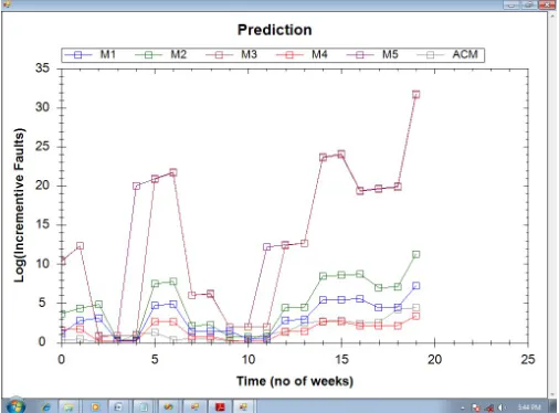
The Figures (Fig 5.1 & Fig 5.2) represents the Fitness and
Prediction graphs of various SRGMs and ACM respectively.
Here the failure data-set Ohba [5] is taken for the comparison purpose.
Fig 5.1 Fitness comparison between Models and ACM with Ohba Dataset
Fig 5.2 Prediction comparison between Models and ACM with Ohba Dataset
6
Conclusion and Future ScopeIn this paper, the Fitness and Prediction of various Software
Reliability Growth Models (SRGMs) can be compared with AdaBoosting based Combinational Model (ACM) with the
help of Maximum likelihood estimation to estimate the model
parameters. From the results, the fitting and prediction
performance of ACM is better compare with individual reliability growth models with real failure data-sets.
The further enhancements those are possible for this, Examining the statistical significance of the estimation and
prediction results of the ACM and Comparing with the other
combination approaches such as Genetic-based Combinational Model (GCM)[9], Dynamic Weighted Combinational Model
(DWCM)[7] etc.
References
[1] Hoang Pham, System Software Reliability. Springer Series in Reliability Engineering..
[2] Jiri Matas and Jan S ochman, AdaBoost, Centre for Machine Perception, Czech Technical University, Prague.
[3] Haifeng Li, Min Zeng, and Minyan Lu, “Exploring AdaBoosting Algorithm for Combining Software Reliability Models”,ISSRE 2009.
[4] X. Cai, M. R. Lyu. Software Reliability Modeling with Test Coverage Experimentation and Measurement with a Fault-Tolerant Software Project. ISSRE, 2007: 17-26
[5] C. Y. Huang, S. Y. Kuo and M. R. Lyu. An assessment of testing-effort dependent software reliability growth models. IEEE Transactions on Reliability, 2007, 56(2): 198-211
[6] Lyu, M. R, Nikora, A. Applying Reliability Models More Effective. IEEE Software, 1992, 9(4): 43-52
[7] Y. S. Su, C. Y. Huang. Neural-network based approaches for software reliability estimation using dynamic weighted combinational models. The Journal of Systems and Software, 2007, 80: 606-615
©2012
7
[9] Eduardo Oliveira Costa, Silvia R. Vergilio, Aurora Pozo, Gustavo Souza.Modeling software reliability growth with Genetic Programming. ISSRE, 2005: 1-10
[10]Artur Ferreira, Survey on Boosting algorithms for supervised and semi-supervised learning. Institute of Telecommunications.
[11] Aasia Quyoum, Mehraj – Ud - Din Dar, Improving Software Reliability using Software Engineering Approach, International Journal of Computer Applications (0975
– 8887) Volume 10– No.5, November 2010.
[12] S. Yamada, J. Hishitani, and S. Osaki, “Software reliability growth model with Weibull testing effort: a model and application” , IEEE Trans. Reliability, vol. R-42, pp. 100–105, 1993.