Simulating future precipitation extremes in a complex Alpine catchment

(1)

Nat. Hazards Earth Syst. Sci., 13, 263–277, 2013 www.nat-hazards-earth-syst-sci.net/13/263/2013/ doi:10.5194/nhess-13-263-2013

EGU Journal Logos (RGB)

Advances in

Geosciences

Open Access

Natural Hazards

and Earth System

Sciences

Open Access

Annales

Geophysicae

Open Access

Nonlinear Processes

in Geophysics

Open Access

Atmospheric

Chemistry

and Physics

Open Access

Atmospheric

Chemistry

and Physics

Open Access Discussions

Atmospheric

Measurement

Techniques

Open Access

Atmospheric

Measurement

Techniques

Biogeosciences

Open Access Open Access

Biogeosciences

Discussions

Climate

of the Past

Climate

of the Past

Discussions

Earth System

Dynamics

Earth System

Dynamics

Discussions

Geoscientific

Instrumentation

Methods and

Data Systems

Open Access

_{Geoscientific}

Instrumentation

Methods and

Data Systems

Geoscientific

Model Development

Geoscientific

Model Development

Discussions

Hydrology and

Earth System

Sciences

Open Access

Hydrology and

Earth System

Sciences

Ocean Science

Discussions

Solid Earth

Discussions

The Cryosphere

Natural Hazards

and Earth System

Sciences

Open Access

Discussions

Simulating future precipitation extremes in a complex

Alpine catchment

C. Dobler1,2, G. B ¨urger3,4, and J. St¨otter1,2

1_{Institute of Geography, University of Innsbruck, Innrain 52, Innsbruck, Austria}

2_{alpS – Centre for Climate Change Adaptation Technologies, Grabenweg 68, Innsbruck, Austria} 3_{Pacific Climate Impact Consortium, University of Victoria, 2489 Sinclair Road, Victoria, Canada}

4_{Institute of Earth and Environmental Science, University of Potsdam, Karl-Liebknecht-Str. 24-25, Potsdam-Golm, Germany}

Correspondence to: C. Dobler ([email protected])

Received: 27 October 2011 – Published in Nat. Hazards Earth Syst. Sci. Discuss.: – Revised: 30 November 2012 – Accepted: 10 December 2012 – Published: 8 February 2013

Abstract. The objectives of the present investigation are

(i) to study the effects of climate change on precipitation ex-tremes and (ii) to assess the uncertainty in the climate pro-jections. The investigation is performed on the Lech catch-ment, located in the Northern Limestone Alps. In order to estimate the uncertainty in the climate projections, two statis-tical downscaling models as well as a number of global and regional climate models were considered. The downscaling models applied are the Expanded Downscaling (XDS) tech-nique and the Long Ashton Research Station Weather Gen-erator (LARS-WG). The XDS model, which is driven by an-alyzed or simulated large-scale synoptic fields, has been cal-ibrated using ECMWF-interim reanalysis data and local sta-tion data. LARS-WG is controlled through stochastic param-eters representing local precipitation variability, which are calibrated from station data only. Changes in precipitation mean and variability as simulated by climate models were then used to perturb the parameters of LARS-WG in order to generate climate change scenarios. In our study we use cli-mate simulations based on the A1B emission scenario. The results show that both downscaling models perform well in reproducing observed precipitation extremes. In general, the results demonstrate that the projections are highly variable. The choice of both the GCM and the downscaling method are found to be essential sources of uncertainty. For spring and autumn, a slight tendency toward an increase in the intensity of future precipitation extremes is obtained, as a number of simulations show statistically significant increases in the in-tensity of 90th and 99th percentiles of precipitation on wet days as well as the 5- and 20-yr return values.

1 Introduction

Global warming may cause an increase of the atmospheric water vapor content and an intensification of the global hydrological cycle (Solomon et al., 2007; O’Gorman and Schneider, 2009). Precipitation extremes may increase in fre-quency and intensity over many areas of the globe (Sun et al., 2007; Allan and Soden, 2008), with substantial consequences for a variety of socio-economic systems (e.g. Easterling et al., 2000; Diffenbaugh et al., 2005).

In the Alps, precipitation is among the major controlling meteorological variables for human–environment systems. Through its triggering effect, precipitation may be seen as the key variable for specific natural hazard processes, i.e. for flash floods (e.g. Frei and Sch¨ar, 1998; Beniston, 2007), de-bris flow (e.g. Chiarle et al., 2007; Szymczak et al., 2010), landslides (e.g. Raetzo et al., 2002; Crosta et al., 2004), hail (e.g. Vinet, 2001) and avalanches (e.g. Martin et al., 2001). In the period from 1982 to 2005, natural hazard pro-cesses caused economic losses in the range of C57 billion in the Alps (Agrawala, 2007). Potential future changes in the frequency and magnitude of precipitation extremes may have serious impacts on ecological, economic and sociolog-ical systems. Consequently, studying the effects of climate change on precipitation extremes is of high societal and eco-nomic relevance.

Despite the high significance of this topic for the Alps, in-vestigations on climate change impacts on precipitation ex-tremes have been very limited so far. Beniston (2006) re-ported a considerable increase in the frequency of heavy

(2)

precipitation events in parts of Switzerland during autumn and winter, while Smiatek et al. (2009) found an increase in the frequency of high precipitation amounts for all over the Alps in winter only. According to Frei et al. (2006) and Schmidli et al. (2007), precipitation extremes are projected to increase north of about 45◦N in winter, whereas there is an insignificant change or a decrease south of it. However, most of these studies have only used one General Circula-tion Model (GCM) and thus, the results only cover a small range of possible changes. Furthermore, most of these inves-tigations were performed on a scale compatible with the grid spacing of Regional Climate Models (RCMs), and thus, the obtained results can only give an incomplete picture of pos-sible changes at local scales. But, as changes in precipitation are expected to vary significantly on small horizontal scales within complex regions like the Alps (Solomon et al., 2007), investigations on more detailed scales are very relevant.

GCMs are the only physically based tools to assess changes in climate resulting from increasing atmospheric greenhouse gases in the atmosphere. The models perform well in reproducing the climate on a global to continental scale. However, the horizontal resolution of GCMs is too coarse for investigating processes on regional or even local scales. In recent years, a variety of different techniques have been developed to bridge this scaling gap. The methods can be divided into (i) dynamical downscaling and (ii) statistical downscaling (Fowler et al., 2007). A comprehensive review is given by Maraun et al. (2010).

Dynamical downscaling is based on highly resolved numerical computer models (Regional Climate Models – RCMs), nested into a GCM over a limited region of interest. The higher horizontal resolution of RCMs, typically 25 km or 50 km, captures regional climate processes much better. Statistical downscaling, instead, establishes an empirical re-lationship between large-scale fields (predictors) and local-scale variables (predictands) (Maraun et al., 2010). The pro-cess is based on the following assumptions for suitable pre-dictors: (i) the predictors are well simulated by the GCMs, (ii) the statistical relationship remains valid in a changed cli-mate, and (iii) the predictors incorporate the future climate change signal (Wilby et al., 2004; Benestad et al., 2008). According to Rummukainen (1997), the variety of statisti-cal downsstatisti-caling methods can be divided into two fundamen-tal approaches, namely Perfect-Prognosis (Perfect-Prog) and Model Output Statistics (MOS). Perfect-Prog is based on a calibration between observed large-scale atmospheric data and observed local-scale data, whereas MOS is calibrated on model output and observed local-scale data (Maraun et al., 2010). Weather generators, which use change factors ob-tained from climate models to generate climate change sce-narios, can be seen as simple MOS (Maraun et al., 2010).

In the recent past, the availability of RCM data led to a tendency to use dynamical rather than statistical downscal-ing. However, in regions with a complex topography the spatial resolution of RCMs is still too coarse to investigate

local climate processes (Engen-Skaugen, 2007). Statistical downscaling is then the only way to generate higher-resolution climate change scenarios and is thus, particularly important for the Alps.

Despite the fact that a number of different statistical down-scaling approaches exist, only a few techniques are reported to downscale extreme events reliably (e.g. Fowler et al., 2007; Tryhorn and DeGaetano, 2011). Modeling extreme events is known to be a difficult challenge, as these phenom-ena lie at the margins of the distribution functions and are often beyond the range of calibration data sets (Harpham and Wilby, 2005; Tolika et al., 2008; Benestad, 2010). So far only a few attempts have been carried out to compare different statistical downscaling techniques with a focus on extreme events.

Bürger and Chen (2005) compared three regression-based statistical downscaling techniques: randomization, inflation and Expanded Downscaling (XDS). The obtained results were quite diverse, highlighting that the choice of the down-scaling approach is a considerable source of uncertainty. Bürger et al. (2012) compared five statistical downscaling methods in simulating climate extremes. The methods con-sidered are: automated regression-based statistical down-scaling, bias correction spatial disaggregation, quantile re-gression neural networks, a weather generator (TreeGen) and XDS. The XDS method was found to perform best, followed by the bias correction and spatial disaggregation and quantile regression neural networks methods. Liu et al. (2011) compared the nonhomogeneous hidden Markov model and the statistical downscaling model SDSM in terms of downscaling precipitation. Both models performed simi-lar in simulating dry- and wet-spell length, while the non-homogeneous hidden Markov model showed better skill in modeling the wet-day precipitation amount. Hundecha and Bárdossy (2008) tested two statistical downscaling tech-niques in their ability to reproduce indices of extremes of daily precipitation and temperature. They found that both methods (multivariate autoregressive model and multiple lin-ear regression) are more reliable during seasons when the lo-cal climate is influenced by large-slo-cale circulation than lolo-cal convective processes.

(3)

C. Dobler et al.: Simulating future precipitation extremes in a complex Alpine catchment 265

Recent studies have shown that projections of single cli-mate model simulations are subjected to large uncertainty (Maurer and Duffy, 2005), which can result from three main sources: (i) emission scenario, (ii) the GCM and (iii) the downscaling technique (e.g. Maurer, 2007). According to D´equ´e et al. (2011), the uncertainty from GCM structure is by far the largest source of uncertainty in climate change pro-jections. Other studies associate large uncertainty with the choice of the downscaling method (e.g. Frei et al., 2006; Schmidli et al., 2007; Beldring et al., 2008; Chen et al., 2011). In addition, the uncertainties may be amplified by natural climate variability (e.g. Booij, 2005; Maraun et al., 2010), especially when focusing on extreme events. Hawkins and Sutton (2011) showed that for decadal means of sea-sonal mean precipitation, internal variability is found to be the most important uncertainty source for lead times up to 30 yr. Model uncertainty is the dominant source for longer lead times, while scenario uncertainty is found to be negligi-ble for all lead times. However, as stated by Willems and Vrac (2011), good practice in climate impact assessments would involve an assessment of the uncertainty in the cli-mate projections. A rough estimation of the overall uncer-tainty can be achieved by using multi-model ensembles con-sisting of different climate models as well as different down-scaling techniques (Hanel and Buishand, 2012).

In this investigation, uncertainty due to the use of GCM and the downscaling technique is assessed. Downscaling is accomplished using two different statistical downscaling models: (i) Expanded Downscaling (XDS, Bürger, 1996) and (ii) the Long Ashton Research Station Weather Generator (LARS-WG, Semenov and Barrow, 1997). Recently, both techniques have been applied in several studies focusing on extreme events (e.g. Mavromatis and Hansen, 2001; Menzel and Bürger, 2002; Qian et al., 2004; Dibike and Coulibaly, 2005; Scibek and Allen, 2006; Semenov, 2007, 2008; Bürger et al., 2009). Comparative studies with other downscaling techniques have shown that both methods have significant skill in reproducing observed precipitation extremes (e.g. Bürger and Chen, 2005; Qian et al., 2008; Hashmi et al., 2011; Bürger et al., 2012). XDS is a Perfect-Prog approach that is based on regression while LARS-WG, instead, is a change factor-conditioned weather generator and is known as simple MOS (Maraun et al., 2010). The XDS technique is applied to downscale GCM output, whereas LARS-WG is used to downscale RCM output. Thus, both techniques are fundamentally different approaches. However, these differ-ences are explicitly desired, because it seems to be very rele-vant to analyse climate change signals simulated by two dif-ferent approaches, as aimed at in the present study. Besides the application of these two different statistical downscaling techniques, a number of GCMs and RCMs are used to assess the range of uncertainty in the climate projections.

The objectives of the present investigation are (i) to refine the understanding of climate change impacts on precipitation extremes in a complex Alpine topography and (ii) to assess

31 Figure 1. Study area with rain gauges

1

2

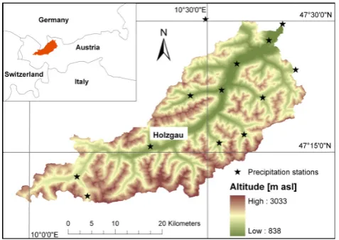
Fig. 1. Study area with rain gauges.

the uncertainty in the climate projections. The study is per-formed on the Lech basin, located in the Northern Limestone Alps. The catchment has already been investigated in a pre-vious application with a focus on climate change impacts on the runoff regime (Dobler et al., 2010). This study reports significant changes in the runoff regime, with an increase of winter runoff and a decrease of summer runoff.

The following section introduces the study area and the available data, followed by a description of the methodology. The results and discussions are presented in Sect. 3. Finally, conclusions are given.

2 Material and methods

2.1 Investigation area

In the present investigation, the Lech watershed located in the Northern Limestone Alps, was selected as the study area. The catchment covers∼1000 km2and can be characterized as a typical Alpine valley with high relief and steep slopes. Figure 1 gives an overview of the study area. The topography is rather complex, with elevation ranging from around 800 m to around 3000 m.

(4)

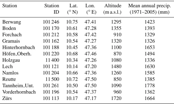
Table 1. Rain gauges.

Station Station Lat. Lon. Altitude Mean annual precip. ID (◦N) (◦E) (m a.s.l.) (1971–2005) (mm)

Berwang 101 246 10.75 47.41 1295 1423

Boden 101 170 10.61 47.28 1355 1393

Forchach 101 212 10.58 47.42 910 1329

Gramais 101 162 10.54 47.27 1320 1326

Hinterhornbach 101 188 10.45 47.36 1100 1653

H¨ofen Oberh. 101 220 10.68 47.46 870 1494

Holzgau 11 400 10.34 47.26 1080 1336

Lech 101 121 10.14 47.20 1480 1630

Namlos 101 204 10.66 47.36 1260 1585

Reutte 11 500 10.72 47.50 850 1385

Tannheim Unt. 101 261 10.50 47.50 1090 1778 Vorderhornbach 101 196 10.54 47.37 960 1362

Z¨urs 101 113 10.17 47.17 1720 1664

maximum temperature is observed in July with +15.2◦C. Between November and March, most precipitation falls as snow in the Lech catchment (see Dobler et al., 2010). Note, however, that our study is entirely based on precipitation ob-servations (apart from temperature); changes in the propor-tion of rain and snow, despite their importance, can therefore not be tackled here.

The Lech watershed is known as a flood-prone region as three extreme floods have occurred there in the recent past (in 1999, 2002 and 2005). For more details about these events see Dobler (2010) or Thieken et al. (2011). Thus, assessing the impacts of climate change on precipitation extremes is of high socio-economic relevance for this region.

2.2 Data

For the present study, thirteen rain gauges have been selected within or close to the catchment. The stations are shown in Fig. 1 and the main characteristics of the stations are given in Table 1. Observed data consisted of daily precipitation data covering the time period from 1971 to 2005. The data was obtained from the Hydrographischer Dienst ¨Osterreich

and the Zentralanstalt f¨ur Meteorologie und Geodynamik (ZAMG). The data were quality controlled, but not homog-enized. Precipitation events with 24-h duration were consid-ered in this study.

Large-scale climate data comprise reanalysis, GCM and RCM data. For the period from 1989 to 2005, daily large-scale reanalysis data was derived from the ERA-interim dataset of the European Centre for Medium-Range Weather Forecasts (ECMWF) (Simmons et al., 2007). The data cover the domain from 40◦–50◦N to 0◦–25◦E. In addition, a num-ber of GCMs and RCMs were selected to simulate current and future climate conditions. Table 2 provides an overview of the different climate simulations used in this work.

For the two GCMs, i.e. ECHAM5 and HadGEM2, an en-semble of three integrations was available with different ini-tial conditions. Ensemble integrations are very helpful when focusing on extreme events, as interannual climate variabil-ity can be better assessed. Following the studies of Frei et al. (2006) and Tolika et al. (2008), the ensemble members were treated as one 90-yr experiment for the present and future scenario. The RCMs with a horizontal resolution of ∼25 km were obtained from the ENSEMBLES project of the European Union (EU; http://ensemblesrt3.dmi.dk/). In this study, the output of nine individual RCM experiments was utilized using seven different RCMs and four GCMs. The output of the two GCMs (ECHAM5, HadGEM2) was down-scaled using the XDS model, while the output of the nine different GCM–RCM combinations was downscaled using LARS-WG.

All climate simulations are forced with the Special Re-port on Emission Scenario (SRES) A1B (Nakicenovic et al., 2000). The A1B scenario is a mid-range scenario in terms of global greenhouse gas emissions. From all simulations the time slices from 1971 to 2000, considered as reference pe-riod, and from 2071 to 2100, as future scenario, were ex-tracted.

2.3 Statistical analysis

2.3.1 Indices

(5)

Table 2. Selected GCMs and RCMs.

GCM RCM Resolution Ensemble Statistical Abbreviation members Downscaling

ECHAM5 – 250 km 3 XDS EH5 XDS

HadGEM2 – 250 km 3 XDS HG2 XDS

HadCM3Q0 CLM 25 km – LARS-WG HC3 CLM LWG

HadCM3Q0 HadRM3Q0 25 km – LARS-WG HC3 HR3 LWG

ARPEGE HIRHAM 25 km – LARS-WG ARP HIR LWG

ECHAM5 RACMO 25 km – LARS-WG EH5 RAC LWG

ECHAM5 REMO 25 km – LARS-WG EH5 REM LWG

ECHAM5 RCA 25 km – LARS-WG EH5 RCA LWG

ECHAM5 HIRHAM 25 km – LARS-WG EH5 HIR LWG

ECHAM5 REGCM 25 km – LARS-WG EH5 REG LWG

BCM RCA 25 km – LARS-WG BCM RCA LWG

Model origins:

ECHAM5, REMO – Max-Planck-Institute for Meteorology (MPI), HadGEM2, HadCM3Q0, HadRM3Q0 – Met Office Hadley Centre (HC), CLM – Swiss Institute of Technology (ETHZ), HIRHAM – Danish Meteorological Institute (DMI), RACMO – Royal Netherlands Meteorological Institute (KNMI), RCA – Swedish Meteorological and Hydrological Institute (SMHI), ARPEGE – Meteo-France, BCM – University of Bergen

In order to assess precipitation events with return peri-ods of 5 and 20 yr, a generalized extreme value (GEV) dis-tribution was applied. The GEV disdis-tribution has been used extensively for a variety of applications in hydrology, clima-tology or meteorology (e.g. Frei et al., 2006; Beniston et al., 2007; Buonomo et al., 2007). It is defined as (Eq. 1):

F (x)=exp (

−

1+κ _x₋_ς

α

−1_κ)

, (1)

whereς,α, andκ are the location, scale and shape param-eter, respectively.F (x)is defined for

x:1+κ x−_ας>0 , where−∞< ς <∞,α >0 and−∞< κ <∞. In the case ofκ <0,κ=0 andκ >0, the well-known Weibull, Gumbel and Fr´equet distributions are obtained (e.g. Russo and Sterl, 2012). In this study, we analysed the data using a block max-ima approach (Coles, 2001). The block maxmax-ima approach is a well-established statistical framework in which the single highest daily precipitation amount over the entire year or sea-son is selected.

The GEV parameters were estimated using the Maximum-Likelihood method. Finally, the assumption if the GEV dis-tribution could be used was tested with the Kolmogorov– Smirnov test, based on a significance level of 5 %. The test indicates if the GEV distribution is a reasonable approxima-tion of the distribuapproxima-tion of annual and seasonal precipitaapproxima-tion maxima. Note that the application of the GEV distribution is based on the key assumption that the data is independently and identically distributed (Wehner et al., 2010).

2.3.2 Confidence intervals

A non-parametric bootstrap simulation method was applied to estimate confidence intervals for the 90th and 99th per-centiles as well as for the 5- and 20-yr return values. The

technique is well recognized in climate impact assessments (e.g. Ekstr¨om et al., 2005). Bootstrap samples were gener-ated for each meteorological station by resampling years. Thereby, the original dataset comprising n years was resam-pled with replacements 1000 times in order to generate in-dependent samples of size n. Convergence experiments con-firmed that 1000 samples are sufficient (not shown). The in-dices described in Sect. 2.3.1 were then calculated for each dataset, and the 5th and 95th percentiles were constructed.

In order to generate confidence intervals for the climate change signals, pairs of bootstrap samples from the reference and scenario simulations were resampled and the quotient be-tween scenario and reference simulation was calculated (Frei et al., 2006). When the ratio of 1.0, which corresponds to no change, lies outside the 90 % confidence interval, the differ-ences are statistically significant.

2.4 Statistical downscaling methods

2.4.1 Long Ashton Research Station Weather Generator (LARS-WG)

The Long Ashton Research Station Weather Generator (LARS-WG, version 5.11; http://www.rothamsted.bbsrc.ac. uk/mas-models/larswg.php) was applied to generate daily site-specific climate change scenarios for the meteorological stations illustrated in Fig. 1.

(6)

Table 3. Precipitation indices.

Abbreviation Definition Unit

Q90,Q99 90th and 99th percentiles of distribution function on wet days mm d−1 x1d5,x1d20 Intensity of a precipitation event with a return period of 5 and 20 yr mm d−1

climate conditions, they have been increasingly applied in climate impact assessments in recent years (e.g. Semenov, 2007; Butterworth et al., 2010).

LARS-WG models precipitation occurrence by alternating series of wet and dry days, based on semi-empirical probabil-ity distributions. The amount of precipitation is simulated by a semi-empirical distribution for each month. Semi-empirical distributions are defined as a histogram with several inter-vals (Semenov and Stratonovitch, 2010; Sunyer et al., 2012). For more details see Semenov et al. (1998) or Semenov and Stratonovitch (2010).

In a first step, the parameters of LARS-WG were calcu-lated by analysing observed precipitation data from the pe-riod 1971 to 2000. The calibrated parameters were then used by LARS-WG to generate synthetic weather series of 100-yr for each site. A long time series allows a better assess-ment of climate extremes as differences between observed and simulated series do not result from the short sampling period (Qian et al., 2004). The performance of the weather generator was evaluated by comparing the synthetically pro-duced 100-yr simulations with observations. In a second step, changes in mean and variability of precipitation as simulated by the RCMs were used to adjust the calibrated parameters of LARS-WG. Therefore, relative changes in monthly precipi-tation as well as monthly shifts in wet and dry series were calculated from the reference simulation (1971 to 2000) and the future scenario (2071 to 2100) of each RCM. The semi-empirical distributions for the future were obtained from the present distribution by multiplying the intervals of the his-togram using the change factors (e.g. Semenov, 2007; Sunyer et al., 2012). A detailed description how the new parameters are generated is given by Semenov (2007).

It has to be noted, that LARS-WG is calibrated on ob-served station data only. Thus, in contrast to XDS, the cal-ibration and reference simulation is identical for LARS-WG. As the future scenarios refer to the reference simulation, we decided to present the performance of the reference sim-ulation of LARS-WG (denoted by OBS LWG) in Sect. 3 together with the downscaled reference simulations using XDS.

2.4.2 Expanded Downscaling (XDS)

XDS is a statistical downscaling technique which belongs to the group of regression methods. It was developed by B¨urger (1996) and has been applied in a variety of applica-tions in recent years, e.g. flood risk assessment (Menzel and

B¨urger, 2002) or flood forecast (B¨urger, 2009). In this study, XDS was applied to downscale GCMs output to finer spatial resolution.

XDS is based on establishing an empirical relationship between large-scale variables x, the “predictors”, and the local-scale variablesy, the so-called “predictands”. In gen-eral, XDS follows the concept of multiple linear regression (MLR) by minimizing the least square error. The main weak-ness of MLR is that it reduces the local climate variability significantly, which is important for a realistic simulation of extreme events. In contrast to classical regression, XDS ex-plicitly preserves local climate variability by adding a side condition so that local covariance is retained. Thus, XDS is found as the matrix Q that minimizes the least square error under the constraining side condition that the local covari-ance is preserved (Eq. 2). Although this leads to a larger mean error compared to MLR, extreme events are simulated much better by XDS. It is important to note that the esti-mation of XDS is entirely done in the normalized domain, which can be achieved for any random variable by means of the probability integral transform (probit). Therefore both, the annual cycle and the statistics of extremes, are mainly defined through the estimated probit parameters. A full de-scription of the XDS technique is given by B¨urger (1996) or B¨urger et al. (2009).

XDS = argmin Q

kxQ−yk subj. toQ0x0xQ=y0y (2)

(7)

0 10 20 30 40

01.01.2005 01.02.2005 01.03.2005 01.04.2005 01.05.2005 01.06.2005

prec

ipitat

ion

[mm/day

] _observed

ECMWF_XDS

Fig. 2. Observed and statistically downscaled precipitation averaged over the entire catchment area from 1 January 2005 to 30 June 2005. The XDS model is forced using ECMWF reanalysis data (denoted by ECMWF XDS).

It has to be noted that LARS-WG and XDS were calibrated on different time periods. Using the same period was not possible, as on the one hand, the period 1989–2000 seems to be too short for a reliable calibration of LARS-WG as at least 30-yr of data are typically used for the simulation of extremes (e.g. Semenov, 2008; Qian et al., 2008). This data shortage affects XDS in the same way but to a lesser extent, since that model is more process-based and requires “only” the sufficient sampling and learning of the most relevant syn-optic conditions. On the other hand, the fact that ECMWF data are not available before 1989 restricts the potential cali-bration period for XDS; note that after the completion of this paper the ECMWF data set was extended to the year 1979 (Dee et al., 2011). Although other reanalysis sets with longer time series were available (e.g. those of NCEP), we selected the ERA-interim data because of their higher quality.

2.4.3 Calibration and validation of XDS

Figure 2 gives an example of the performance of the XDS model driven with ECMWF data during the validation pe-riod. In general, observed precipitation is reproduced fairly well by the XDS model. However, the figure indicates that some over- and underestimations are evident, especially in the case of the most extreme events. For daily areal precip-itation, which is defined as the daily mean of all precipita-tion staprecipita-tions, the correlaprecipita-tion coefficient between observed and simulated time series constitutes 0.78 for the calibra-tion period (1989 to 2000) and 0.76 for the validacalibra-tion period (2001 to 2005). Note that five years are quite short for a vali-dation period of extreme events, but at least a decade of daily data is necessary to calibrate the XDS model.

Figure 3 shows a comparison of the percentiles of ob-served and simulated precipitation series, based on the period from 1989 to 2005. In general, XDS performs very well in simulating precipitation extremes. Even for the highest per-centiles, i.e. 99th percentile, a good agreement between ob-servation and simulation is obtained.

XDS shows a slight seasonal bias with underestimat-ing precipitation events of more than around 30 mm day−1 in spring. In contrast, slight overestimations are evident in

Fig. 3. Percentile-percentile plots showing observed versus down-scaled precipitation on wet days (>1 mm day−1)using XDS for (a) the calibration (1989–2000) and (b) the validation period (2001– 2005). The XDS model is forced using ECMWF reanalysis data.

winter. In autumn, the XDS model was found to perform best. However, also other studies using Perfect-Prog tech-niques like XDS report that these models perform gener-ally better during autumn and winter than during spring and summer (e.g. Harpham and Wilby, 2005; Hundecha and B´ardossy, 2008; Tolika et al., 2008). This can be explained by the fact that during autumn and winter, the local climate depends more on the large-scale circulation, while during spring and summer local convective processes are important (Hundecha and B´ardossy, 2008).

3 Results and discussion

(8)

34 1

2

Figure 4: (a) 90-% and (b) 99-% percentiles of observation (1971-2000) and reference 3

simulations (EH5_XDS, HG2_XDS, OBS_LWG; 1971-2000). Vertical lines indicate 90-% 4

bootstrap confidence intervals. 24-h precipitation events averaged over the Lech catchment 5

are shown. 6

7

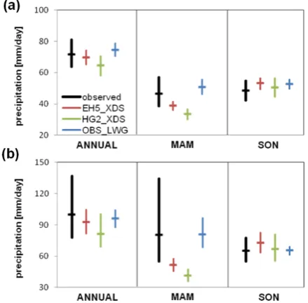
Fig. 4. (a) 90th and (b) 99th percentiles of observation (1971–2000) and reference simulations (EH5 XDS, HG2 XDS, OBS LWG; 1971–2000). Vertical lines indicate 90% bootstrap confidence in-tervals. 24-h precipitation events averaged over the Lech catchment are shown.

3.1 Evaluation of reference simulations

Figure 4 illustrates the 90th and 99th percentiles of precipita-tion events, based on the observed time series and the refer-ence simulations using the two downscaling techniques. Note that in the case of XDS, the precipitation variability is de-rived from the GCM control simulations, while for LARS-WG, the variability is obtained from observations.

In general, the reference simulations agree fairly well with observations. Even for the 99th percentile, which cor-responds to the amount of daily precipitation exceeded with a probability of 0.01, a good agreement between observation and reference simulations is obtained. The figure reveals that all reference simulations reproduce the seasonal cycle of the two percentiles very well, with maximum values during sum-mer and lower values during spring.

The performance of the EH5 XDS and HG2 XDS ref-erence simulations varies with seasons, whereas the per-formance of OBS LWG is similar for all seasons. Both EH5 XDS and HG2 XDS underestimate the 90th percentile in summer and the 99th percentile in spring, respectively, whereas they slightly overestimate the 99th percentile in win-ter. However, when comparing the results of Figs. 3 and 4, it can be seen that the agreement between observation and the XDS simulations driven with GCM data is similar to the agreement between observation and XDS simulation driven with ECMWF data. Thus, the quality of both GCMs in sim-ulating the selected predictors seems to be relatively good.

OBS LWG slightly overestimates the 90th and 99th per-centiles in all seasons. The largest bias for OBS LWG is found for the 99th percentile in summer.

Fig. 5. (a) 5-yr and (b) 20-yr return values for observation (1971–2000) and reference simulations (EH5 XDS, HG2 XDS, OBS LWG; 1971–2000). Vertical lines indicate 90% bootstrap con-fidence intervals. 24-h precipitation events averaged over the Lech catchment are shown.

Figure 5 shows the performance of the reference simula-tions in reproducing the 5- and 20-yr return values. Although the analysis was made for the whole year and all seasons, here only the results for the year as well as for spring and autumn are presented, as these are the periods with the most pronounced deviations.

Again, the seasonal variations of the 5- and 20-yr return values are captured fairly well by the reference simulations. Except the HG2 XDS simulation in spring, all reference sim-ulations fall within the 90% confidence intervals of obser-vation, showing that the downscaling techniques perform well in reproducing observed precipitation extremes. The EH5 XDS and HG2 XDS simulations underestimate the 5-and 20-yr return values in spring, whereas they perform well in autumn. For OBS LWG, a good performance in simulat-ing the 5- and 20-yr return values is found in both seasons.

(9)

36 1

2

Figure 6: Ratio between scenario (2071-2100) and reference (1971-2000) simulations for (a) 3

90-% and (b) 99-% percentiles. Vertical lines indicate 90-% bootstrap confidence interval. 4

The results are statistically significant when the ratio of 1.0 lies outside the 90% confidence 5

interval. 24-h precipitation events averaged over the Lech catchment are shown. 6

7

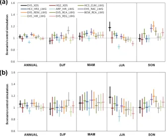
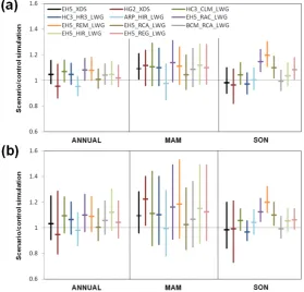
Fig. 6. Ratio between scenario (2071–2100) and reference (1971–2000) simulations for (a) 90th and (b) 99th percentiles. Vertical lines indicate 90 % bootstrap confidence interval. The results are statistically significant when the ratio of 1.0 lies outside the 90 % confidence interval. 24-h precipitation events averaged over the Lech catchment are shown.

Landesregierung, 1999; Meier, 2002). The inclusion of such extreme events in the sample considerably modifies the ex-treme value distribution and thus has a significant impact on the calculation of the 20-yr return value.

In summary, the reference simulations agree fairly well with observations, even for extreme events such as the 20-yr return value. Compared with the results presented in nu-merous other studies using different statistical downscaling techniques (e.g. Harpham and Wilby, 2005; Wetterhall et al., 2009; Quintana-Segu´ı et al., 2011), observed precipita-tion extremes could be reproduced very well in this study. In the case of XDS, this can be explained by the fact that this technique has been particularly designed to simulate cli-mate extremes. XDS preserves the local clicli-mate variabil-ity by adding the side condition that local covariance is re-tained (see Sect. 2.4.2). Thus, extreme events are simulated much better by XDS than for example by multiple linear re-gression (B¨urger, 1996). LARS-WG approximates daily pre-cipitation with a semi-empirical distribution consisting of a histogram with 23 intervals (Semenov and Stratonovitch, 2010). A semi-empirical distribution is very flexible, does not assume a particular theoretical distribution function and can approximate a wide range of different distributions (e.g. Semenov et al., 1998; Semenov, 2008). The application of a

semi-empirical distribution can thus improve the simulation of extreme events (e.g. Qian et al., 2004).

3.2 Climate change scenarios

We now study the impacts of climate change on extreme precipitation events by comparing the reference simulation (1971–2000) with the scenario simulation (2071–2100) of each climate run. The future scenario is based on the A1B emission scenario.

(10)

37 1

2

Figure 7: Ratio between scenario (2071-2100) and reference (1971-2000) simulations for (a) 3

5-year return value and (b) 20-year return value. Vertical lines indicate 90-% bootstrap 4

confidence interval. The results are statistically significant when the ratio of 1.0 lies outside 5

the 90% confidence interval. 24-h precipitation events averaged over the Lech catchment are 6

shown. 7

Fig. 7. Ratio between scenario (2071–2100) and reference (1971–2000) simulations for (a) 5-yr return value and (b) 20-yr return value. Vertical lines indicate 90 % bootstrap confidence interval. The results are statistically significant when the ratio of 1.0 lies outside the 90 % confidence interval. 24-h precipitation events averaged over the Lech catchment are shown.

The uncertainty in the projection is assessed by calculating the difference between the maximum and minimum of the future precipitation projections. In general, the uncertainty for both percentiles is comparatively small during winter and spring and relatively large during summer and autumn. This is in consensus with the findings of Schmidli et al. (2007), who obtained larger uncertainty in summer than in winter, too, when applying different statistical and dynamical down-scaling methods over the European Alps.

The largest uncertainty is found for the 90th percentile in summer, in which the EH5 XDS simulation shows a statistically significant increase (+18 %), whereas the ARP HIR LWG simulation indicates a statistically signifi-cant decrease (−15 %). Except the ARP HIR LWG simula-tion, which indicates statistically significant decreases for the 90th and 99th percentiles in summer and the 90th percentile for the whole year, and the EH5 REG LWG simulation for the 90th percentile in summer, all remaining simulations in-dicate either insignificant changes or statistically significant increases in all seasons.

Figure 7 illustrates changes in the intensity of 5- and 20-yr return values. Table 4 summarizes the changes for the selected indices. As can be seen, the confidence intervals generated by the bootstrapping approach are relatively wide and increase with the rarity of the event. This makes it very

difficult to detect statistically significant changes in the case of extreme events. Although a number of climate scenarios shows an increase in the intensity of 5- and 20-yr return val-ues, most of these changes are statistically not significant (see Table 4).

(11)

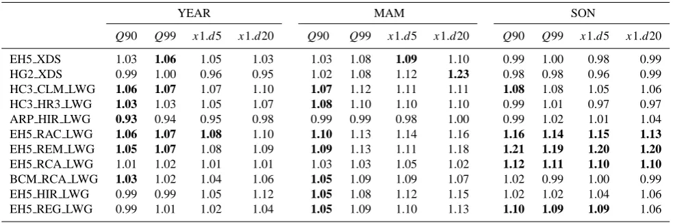
Table 4. Ratio between scenario and reference simulations for the 90th and 99th percentiles as well as for the 5- and 20-yr return values. 24-h precipitation events averaged over the Lech catchment are shown.

YEAR MAM SON

Q90 Q99 x1.d5 x1.d20 Q90 Q99 x1.d5 x1.d20 Q90 Q99 x1.d5 x1.d20

EH5 XDS 1.03 1.06 1.05 1.03 1.03 1.08 1.09 1.10 0.99 1.00 0.98 0.99

HG2 XDS 0.99 1.00 0.96 0.95 1.02 1.08 1.12 1.23 0.98 0.98 0.96 0.99

HC3 CLM LWG 1.06 1.07 1.07 1.10 1.07 1.12 1.11 1.11 1.08 1.08 1.05 1.06

HC3 HR3 LWG 1.03 1.03 1.05 1.07 1.08 1.10 1.10 1.10 0.99 1.01 0.97 0.97

ARP HIR LWG 0.93 0.94 0.95 0.98 0.99 0.99 0.98 1.00 0.99 1.02 1.01 1.04

EH5 RAC LWG 1.06 1.07 1.08 1.10 1.10 1.13 1.14 1.16 1.16 1.14 1.15 1.13

EH5 REM LWG 1.05 1.07 1.08 1.09 1.09 1.13 1.11 1.18 1.21 1.19 1.20 1.20

EH5 RCA LWG 1.01 1.02 1.01 1.01 1.03 1.03 1.05 1.02 1.12 1.11 1.10 1.10

BCM RCA LWG 1.03 1.02 1.04 1.06 1.05 1.09 1.09 1.07 1.02 0.99 1.00 0.99

EH5 HIR LWG 0.99 0.99 1.05 1.12 1.05 1.08 1.12 1.15 1.02 1.02 1.04 1.06

EH5 REG LWG 0.99 1.01 1.02 1.04 1.05 1.09 1.10 1.13 1.10 1.09 1.09 1.06

Bold numbers indicate statistically significant changes (see Sect. 2.3.2).

The projected increase in precipitation extremes agrees with theoretical considerations (Clausius-Clapeyron rela-tion) that the maximum moisture content of the atmosphere increases with approximately 7 % for a 1◦C rise in tempera-ture (e.g. Solomon et al., 2007). Under a constant relative hu-midity, increases in temperature result in increases in water vapor at the same rate (e.g. Solomon et al., 2007). Hence, it is expected that precipitation extremes increase as the climate warms (Allan and Soden, 2008; O’Gorman and Schneider, 2009; Lenderink et al., 2011).

Finally, we analyse the range of uncertainty resulting from different sources. Analysis of different GCMs downscaled by the same statistical downscaling technique reveals that the GCM is an essential source of uncertainty. As can be seen in Fig. 6a, large differences between the EH5 XDS and HG2 XDS simulations are obtained in summer. While the EH5 XDS simulation indicates an increase in the intensity of the 90th percentile of 20 % in summer, the HG2 XDS simu-lation shows no change. Similar results were found in a vari-ety of studies, e.g. D´equ´e et al. (2011). Beside uncertainty resulting from the GCM, dynamical and statistical down-scaling contributes to considerable uncertainty in the projec-tions. For example, changes between−1 % (EH5 XDS) and +21 % (EH5 REM LWG) in the intensity of the 90th per-centile of precipitation on wet days in autumn are obtained for the same GCM downscaled by different techniques (see Fig. 6a).

4 Conclusions

The main objectives of this investigation were (i) to study the impacts of climate change on precipitation extremes and (ii) to assess the range of uncertainty in the climate projec-tions by applying two statistical downscaling techniques as well as multiple GCMs and RCMs. The Lech catchment,

located in the Northern Limestone Alps, was selected as the study area.

In general, downscaling precipitation extremes is a chal-lenging task and is subjected to large uncertainty. Recently, several investigations have reported large model biases when focusing on precipitation extremes (e.g. Smiatek et al., 2009). In this investigation, two well-recognized downscal-ing techniques were selected to simulate precipitation ex-tremes in a complex Alpine topography. The models are completely different in their underlying concepts: XDS is a Perfect-Prog approach whereas LARS-WG belongs to MOS. In the case of LARS-WG, changes in monthly means derived from climate models are used to alter the calibrated param-eters. Hence, in contrast to XDS, LARS-WG does not di-rectly use large-scale atmospheric data. However, these dif-ferent characters of the two techniques are fully intended in order to assess the spread of climate change signals. The re-sults showed that both downscaling models performed very well in reproducing observed precipitation extremes. The bi-ases of all simulations were within an acceptable range, even for very rare events, e.g that one with a 20-yr return period. Thus, XDS and LARS-WG are valuable tools to study the effects of climate change on precipitation extremes on local scales.

(12)

XDS is that site-specific scenarios can be produced very easy, which makes the technique attractive for a common user, while the main disadvantage is that it cannot produce spa-tially correlated climate information, which is necessary in a variety of applications.

A special focus of this study was on assessing the un-certainty in the climate projections. Unun-certainty originating from GCMs and downscaling was considered. The results demonstrate that the climate projections show large varia-tions in the magnitude of the projected climate change sig-nals. In some cases, the simulated changes even pointed towards different directions. Thus, it is emphasized to in-clude and assessment of uncertainty in climate impact assess-ments in future studies, according to the recommendation of Willems and Vrac (2011). Otherwise, the reliability of such studies will be decisively reduced.

Although the present study addressed the main sources of uncertainty, only a rough estimation of the overall un-certainty in the climate projections could be given. This is mainly due to a comparatively small number of different GCMs and downscaling techniques selected in this inves-tigation. However, beside uncertainty related to the GCM, the results of this study also demonstrate that downscaling is an important source of uncertainty. This has to be taken into consideration in future studies.

Nevertheless, when studying the impacts of climate change on precipitation extremes in the Lech basin, a va-riety of interesting findings were obtained. The majority of simulations indicate statistically insignificant changes or sta-tistically significant increases during all seasons. Compara-tively pronounced climate change signals could be obtained for spring and autumn as several climate simulations indi-cate statistically significant increase in the intensity 90th and 99th percentiles of precipitation on wet days and the 5- and yr return values. In autumn, for example, a present 20-yr return event could occur every 6 20-yr in the future scenario and thus, the frequency could increase by a factor of up to 3.3. However, it should be noticed, that due to a strong spa-tial variability of precipitation in the Alps, the results of this study may not be valid for other Alpine catchments.

Recently, Dobler et al. (2010) assessed climate change im-pacts on the runoff regime of the same catchment. This study reports that climate change is expected to strongly affect the hydrological conditions in the basin, with decreases in runoff during summer and increases in winter. However, compared to assessing climate change impacts on average conditions, studying changes in extremes is much more difficult and sub-jected to large variability, with little evidence for clear trends.

Acknowledgements. This work is funded by the Austrian Climate and Energy Fund within the program line ACRP (Austrian Climate Research Program). The ENSEMBLES data used in this work was funded by the EU FP6 Integrated Project ENSEMBLES (Contract number 505539) whose support is gratefully acknowledged.

Edited by: M.-C. Llasat

Reviewed by: two anonymous referees

References

Agrawala, S.: Climate Change in the European Alps: Adapting Winter Tourism and Natural Hazard Management, Organisation for Economic Cooperation and Development Publications, Paris, 2007.

Allan, R. P. and Soden, B. J.: Atmospheric Warming and the Am-plification of Precipitation Extremes, Science, 321, 1481–1484, doi:10.1126/science.1160787, 2008.

Amt der Tiroler Landesregierung: Hydrologische ¨Ubersicht Mai 1999, Innsbruck, Austria, 1999.

Beldring, S., Engen-Skaugen, T., Førland, E. J., and Roald, L. A.: Climate change impacts on hydrological processes in Norway based on two methods for transferring regional climate model results to meteorological station sites, Tellus A, 60, 439–450, doi:10.1111/j.1600-0870.2008.00306.x, 2008.

Benestad, R. E.: Downscaling precipitation extremes, Theor. Appl. Climatol., 100, 1–21, doi:10.1007/s00704-009-0158-1, 2010. Benestad, R. E., Hanssen-Bauer, I., and Deliang, C.:

Empirical-statistical downscaling, World Sci., Singapore, 2008.

Beniston, M.: August 2005 intense rainfall event in Switzer-land: Not necessarily an analog for strong convective events in a greenhouse climate, Geophys. Res. Lett., 33, L05701, doi:10.1029/2005gl025573, 2006.

Beniston, M.: Linking extreme climate events and economic im-pacts: Examples from the Swiss Alps, Energy Policy, 35, 5384– 5392, 2007.

Beniston, M., Stephenson, D., Christensen, O., Ferro, C., Frei, C., Goyette, S., Halsnaes, K., Holt, T., Jylh¨a, K., Koffi, B., Palutikof, J., Sch¨oll, R., Semmler, T., and Woth, K.: Future extreme events in European climate: an exploration of regional climate model projections, Climatic Change, 81, 71–95, doi:10.1007/s10584-006-9226-z, 2007.

Booij, M. J.: Impact of climate change on river flooding assessed with different spatial model resolutions, J. Hydrol., 303, 176– 198, 2005.

Buonomo, E., Jones, R., Huntingford, C., and Hannaford, J.: On the robustness of changes in extreme precipitation over Europe from two high resolution climate change simulations, Q. J. Roy. Meteorol. Soc., 133, 65–81, doi:10.1002/qj.13, 2007.

B¨urger, G.: Expanded downscaling for generating local weather scenarios, Climate Res., 7, 111–128, doi:10.3354/cr0007111, 1996.

B¨urger, G.: Dynamically vs. empirically downscaled medium-range precipitation forecasts, Hydrol. Earth Syst. Sci., 13, 1649–1658, doi:10.5194/hess-13-1649-2009, 2009.

B¨urger, G. and Chen, Y.: Regression-based downscaling of spatial variability for hydrologic applications, J. Hydrol., 311, 299–317, 2005.

B¨urger, G., Reusser, D., and Kneis, D.: Early flood warnings from empirical (expanded) downscaling of the full ECMWF En-semble Prediction System, Water Resour. Res., 45, W10443, doi:10.1029/2009wr007779, 2009.

(13)

B¨urger, G., Murdock, T. Q., Werner, A. T., Sobie, S. R., and Can-non, A. J.: Downscaling extremes – an intercomparison of multi-ple statistical methods for present climate, J. Climate, 25, 4366– 4388, doi:10.1175/JCLI-D-11-00408.1, 2012.

Butterworth, M. H., Semenov, M. A., Barnes, A., Moran, D., West, J. S., Bruce, D., and Fitt, L.: North-South divide: contrasting im-pacts of climate change on crop yields in Scotland and England, J. Roy. Soc. Int., 7, 123–130, 2010.

Chen, J., Brissette, F. O. P., and Leconte, R.: Uncertainty of down-scaling method in quantifying the impact of climate change on hydrology, J. Hydrol., 401, 190–202, 2011.

Chiarle, M., Iannotti, S., Mortara, G., and Deline, P.: Recent de-bris flow occurrences associated with glaciers in the Alps, Global Planet. Chang., 56, 123–136, 2007.

Coles, S.: An Introduction to Statistical Modeling of Extreme Val-ues, Springer, New York, 2001.

Crosta, G. B., Chen, H., and Lee, C. F.: Replay of the 1987 Val Pola Landslide, Italian Alps, Geomorphology, 60, 127–146, 2004. Dee, D. P., Uppala, S. M., Simmons, A. J., Berrisford, P., Poli,

P., Kobayashi, S., Andrae, U., Balmaseda, M. A., Balsamo, G., Bauer, P., Bechtold, P., Beljaars, A. C. M., van de Berg, L., Bid-lot, J., Bormann, N., Delsol, C., Dragani, R., Fuentes, M., Geer, A. J., Haimberger, L., Healy, S. B., Hersbach, H., Hólm, E. V., Isaksen, L., K˚allberg, P., Köhler, M., Matricardi, M., McNally, A. P., Monge-Sanz, B. M., Morcrette, J. J., Park, B. K., Peubey, C., de Rosnay, P., Tavolato, C., Thépaut, J. N., and Vitart, F.: The ERA-Interim reanalysis: configuration and performance of the data assimilation system, Q. J. Roy. Meteorol. Soc., 137, 553– 597, doi:10.1002/qj.828, 2011.

D´equ´e, M., Somot, S., Sanchez-Gomez, E., Goodess, C., Jacob, D., Lenderink, G., and Christensen, O.: The spread amongst EN-SEMBLES regional scenarios: regional climate models, driving general circulation models and interannual variability, Clim. Dy-nam., 38, 951–964, doi:10.1007/s00382-011-1053-x, 2011. Dibike, Y. B. and Coulibaly, P.: Hydrologic impact of climate

change in the Saguenay watershed: comparison of downscaling methods and hydrologic models, J. Hydrol., 307, 145–163, 2005. Diffenbaugh, N. S., Pal, J. S., Trapp, R. J., and Giorgi, F.: Fine-scale processes regulate the response of extreme events to global climate change, Proc. Natl. Acad. Sci., 102, 15774–15778, 2005. Dobler, C.: Possible Changes in Flood Frequency in an Alpine Catchment, in: Risk and Planet Earth. Vulnerability, Natural Haz-ards, Integrated Adaptation Strategies, edited by: D¨olemeyer, A., Zimmer, J., and Tetzlaff, G., 88–94, 2010.

Dobler, C., St¨otter, J., and Sch¨oberl, F.: Assessment of climate change impacts on the hydrology of the Lech Valley in northern Alps, J. Water Climate Change, 3, 207–218, 2010.

Easterling, D. R., Meehl, G. A., Parmesan, C., Changnon, S. A., Karl, T. R., and Mearns, L. O.: Climate Extremes: Ob-servations, Modeling, and Impacts, Science, 289, 2068–2074, doi:10.1126/science.289.5487.2068, 2000.

Ekstr¨om, M., Fowler, H. J., Kilsby, C. G., and Jones, P. D.: New es-timates of future changes in extreme rainfall across the UK using regional climate model integrations, 2. Future estimates and use in impact studies, J. Hydrol., 300, 234–251, 2005.

Engen-Skaugen, T.: Refinement of dynamically downscaled pre-cipitation and temperature scenarios, Climatic Change, 84, 365– 382, doi:10.1007/s10584-007-9251-6, 2007.

Fowler, H. J., Blenkinsop, S., and Tebaldi, C.: Linking climate change modelling to impacts studies: recent advances in down-scaling techniques for hydrological modelling, Int. J. Climatol., 27, 1547–1578, doi:10.1002/joc.1556, 2007.

Frei, C. and Sch¨ar, C.: A precipitation climatology of the Alps from high-resolution rain-gauge observations, Int. J. Climatol., 18, 873–900, 1998.

Frei, C., Sch¨oll, R., Fukutome, S., Schmidli, J., and Vidale, P. L.: Future change of precipitation extremes in Europe: Intercompar-ison of scenarios from regional climate models, J. Geophys. Res., 111, D06105, doi:10.1029/2005jd005965, 2006.

Hanel, M. and Buishand, T. A.: Multi-model analysis of RCM simulated 1-day to 30-day seasonal precipitation ex-tremes in the Czech Republic, J. Hydrol., 412–413, 141–150, doi:10.1016/j.jhydrol.2012.09.020, 2012.

Harpham, C. and Wilby, R. L.: Multi-site downscaling of heavy daily precipitation occurrence and amounts, J. Hydrol., 312, 235–255, 2005.

Hashmi, M., Shamseldin, A., and Melville, B.: Comparison of SDSM and LARS-WG for simulation and downscaling of ex-treme precipitation events in a watershed, Stochastic Environ. Res. Risk Assess., 25, 475–484, doi:10.1007/s00477-010-0416-x, 2011.

Hawkins, E. and Sutton, R.: The Potential to Narrow Uncertainty in Regional Climate Predictions, B. Am. Meteorol. Soc., 90, 1095– 1107, doi:10.1175/2009bams2607.1, 2009.

Hawkins, E. and Sutton, R.: The potential to narrow uncertainty in projections of regional precipitation change, Clim. Dynam., 37, 407–418, doi:10.1007/s00382-010-0810-6, 2011.

Hundecha, Y. and B´ardossy, A.: Statistical downscaling of ex-tremes of daily precipitation and temperature and construc-tion of their future scenarios, Int. J. Climatol., 28, 589–610, doi:10.1002/joc.1563, 2008.

Lenderink, G., Mok, H. Y., Lee, T. C., and van Oldenborgh, G. J.: Scaling and trends of hourly precipitation extremes in two different climate zones – Hong Kong and the Netherlands, Hy-drol. Earth Syst. Sci., 15, 3033–3041, doi:10.5194/hess-15-3033-2011, 2011.

Liu, Z., Xu, Z., Charles, S. P., Fu, G., and Liu, L.: Evaluation of two statistical downscaling models for daily precipitation over an arid basin in China, Int. J. Climatol., 31, 2006–2020, doi:10.1002/joc.2211, 2011.

Maraun, D., Wetterhall, F., Ireson, A. M., Chandler, R. E., Kendon, E. J., Widmann, M., Brienen, S., Rust, H. W., Sauter, T., The-meßl, M., Venema, V. K. C., Chun, K. P., Goodess, C. M., Jones, R. G., Onof, C., Vrac, M., and Thiele-Eich, I.: Precipi-tation downscaling under climate change: Recent developments to bridge the gap between dynamical models and the end user, Rev. Geophys., 48, RG3003, doi:10.1029/2009rg000314, 2010. Martin, E., Giraud, G., Lejeune, Y., and Boudart, G.: Impact of a

climate change on avalanche hazard, Ann. Glaciol., 32, 163–167, 2001.

Maurer, E.: Uncertainty in hydrologic impacts of climate change in the Sierra Nevada, California, under two emissions scenarios, Climatic Change, 82, 309–325, doi:10.1007/s10584-006-9180-9, 2007.

(14)

Maurer, E. P. and Hidalgo, H. G.: Utility of daily vs. monthly large-scale climate data: an intercomparison of two statistical downscaling methods, Hydrol. Earth Syst. Sci., 12, 551–563, 10, http://www.hydrol-earth-syst-sci.net/12/551/10/.5194/hess-12-551-2008, 2008.

Mavromatis, T. and Hansen, J. W.: Interannual variability charac-teristics and simulated crop response of four stochastic weather generators, Agr. Forest Meteorol., 109, 283–296, 2001. Meier, I. M.: Leben mit dem Hochwasser, Ausgew¨ahlte

Hochwasserereignisse des 20. Jahrhunderts im Tiroler Lech-tal, in: Innsbrucker Geographische Gesellschaft, Innsbrucker Jahresbericht 2001/2002, 5–29, 2002.

Menzel, L. and B¨urger, G.: Climate change scenarios and runoff response in the Mulde catchment (Southern Elbe, Germany), J. Hydrol., 267, 53–64, 2002.

Nakicenovic, N., Alcamo, J., Davis, G., de Vries, B., Fenhann, J., Gaffin, S., Gregory, K., Gr¨ubler, A., Jung, T. Y., Kram, T., Rovere, E. L. L., Michaelis, L., Mori, S., Morita, T., Pepper, W., Pitcher, H., Price, L., Raihi, K., Roehl, A., Rogner, H.-H., Sankovski, A., Schlesinger, M., Shukla, P., Smith, S., Swart, R., Rooijen, S. V., Victor, N., and Dadi, Z.: Emission Scenarios. A Special Report of Working Group III of the Intergovernmental Panel on Climate Change, Cambridge University press, Cam-bridge, UK, 2000.

O’Gorman, P. A. and Schneider, T.: The physical basis for increases in precipitation extremes in simulations of the 21st-century cli-mate change, Proc. Natl. Aca. Sci., 106, 14773–14777, 2009. Palmer, T. N. and Raisanen, J.: Quantifying the risk of extreme

sea-sonal precipitation events in a changing climate, Nature, 415, 512–514, 2002.

Qian, B., Gameda, S., Hayhoe, H., Jong, R. D., and Bootsma, A.: Comparison of LARS-WG and AAFC-WG stochastic weather generators for diverse Canadian climates, Climate Res., 26, 175– 191, doi:10.3354/cr026175, 2004.

Qian, B., Gameda, S., and Hayhoe, H.: Performance of stochastic weather generators LARS-WG and AAFC-WG for reproducing daily extremes of diverse Canadian climates, Climate Res., 37, 17–33, doi:10.3354/cr00755, 2008.

Quintana-Segu´ı, P., Habets, F., and Martin, E.: Comparison of past and future Mediterranean high and low extremes of precipita-tion and river flow projected using different statistical down-scaling methods, Nat. Hazards Earth Syst. Sci., 11, 1411–1432, doi:10.5194/nhess-11-1411-2011, 2011.

Raetzo, H. R., Lateltin, O. L., Bollinger, D. B., and Tripet, J. T.: Hazard assessment in Switzerland – Codes of Practice for mass movements, B. Eng. Geol. Environ.t, 61, 263–268, doi:10.1007/s10064-002-0163-4, 2002.

Rummukainen, M.: Methods of statistical downscaling of GCM simulations. Reports Meteorology and Climatology 80, Tech. rep., Swedish Meteorological and Hydrological Institute, SE-601 76 Norrkping, Sweden, 1997.

Russo, S. and Sterl, A.: Global changes in seasonal means and ex-tremes of precipitation from daily climate model data, J. Geo-phys. Res., 117, D01108, doi:10.1029/2011jd016260, 2012. Schmidli, J., Goodess, C. M., Frei, C., Haylock, M. R., Hundecha,

Y., Ribalaygua, J., and Schmith, T.: Statistical and dynamical downscaling of precipitation: An evaluation and comparison of scenarios for the European Alps, J. Geophys. Res., 112, D04105, doi:10.1029/2005jd007026, 2007.

Scibek, J. and Allen, D. M.: Modeled impacts of predicted climate change on recharge and groundwater levels, Water Resour. Res., 42, W11405, doi:10.1029/2005wr004742, 2006.

Semenov, M. A.: Development of high-resolution UKCIP02-based climate change scenarios in the UK, Agr. Forest Meteorol., 144, 127–138, 2007.

Semenov, M. A.: Simulation of extreme weather events by a stochastic weather generator, Climate Res., 35, 203–212, doi:10.3354/cr00731, 2008.

Semenov, M. A. and Barrow, E. M.: Use of a stochastic weather generator in the development of climate change scenarios, Climatic Change, 35, 397–414, doi:10.1023/a:1005342632279, 1997.

Semenov, M. A. and Stratonovitch, P.: Use of multi-model en-sembles from global climate models for assessment of climate change impacts, Climate Res., 41, 1–14, doi:10.3354/cr00836, 2010.

Semenov, M. A., Brooks, R. J., Barrow, E. M., and Richardson, C. W.: Comparison of the WGEN and LARS-WG stochastic weather generators for diverse climates, Climate Res., 10, 95– 107, doi:10.3354/cr010095, 1998.

Simmons, A. S., Uppala, D. D., and Kobayashi, S.: ERA-interim: new ECMWF reanalysis products from 1989 onwards, ECMWF Newsletter, 110, 29–35, 2007.

Smiatek, G., Kunstmann, H., Knoche, R., and Marx, A.: Precipita-tion and temperature statistics in high-resoluPrecipita-tion regional climate models: Evaluation for the European Alps, J. Geophys. Res., 114, D19107, doi:10.1029/2008jd011353, 2009.

Solomon, S., Qin, D., Manning, M., Alley, R. B., Berntsen, T.,Bindoff, N. L., Chen, Z., Chidthaisong, A., Gregory, J. M., Hegerl, G. C., Heimann, M., Hewitson, B., Hoskins, B. J., Joos, F., Jouzel, J., Kattsov, V., Lohmann, U., Matsuno, T., Molina, M., Nicholls, N., Overpeck, J., Raga, G., Ramaswamy, V., Ren, J., Rusticucci, M., Somerville, R., Stocker, T. F., Whetton, P.,Wood, R. A., and Wratt, D.: Technical Summary, in: Climate Change 2007: The Physical Science Basis, Contribution of Working Group I to the Fourth Assessment Report of the Intergovernmen-tal Panel on Climate Change, edited by: Solomon, S., Qin, D., Manning, M., Chen, Z., Marquis, M., Averyt, K. B., Tignor, M., and Miller, H. L., Cambridge University Press, UK, 2007. Sun, Y., Solomon, S., Dai, A., and Portmann, R. W.: How Often

Will It Rain?, J. Climate, 20, 4801–4818, doi:10.1175/jcli4263.1, 2007.

Sunyer, M. A., Madsen, H., and Ang, P. H.: A comparison of dif-ferent regional climate models and statistical downscaling meth-ods for extreme rainfall estimation under climate change, Atmos. Res., 103, 119–128, 2012.

Szymczak, S., Bollschweiler, M., Stoffel, M., and Dikau, R.: Debris-flow activity and snow avalanches in a steep watershed of the Valais Alps (Switzerland): Dendrogeomorphic event re-construction and identification of triggers, Geomorphology, 116, 107–114, 2010.

(15)

Tolika, K., Anagnostopoulou, C., Maheras, P., and Vafiadis, M.: Simulation of future changes in extreme rainfall and temperature conditions over the Greek area: A comparison of two statistical downscaling approaches, Global Planet. Chang., 63, 132–151, 2008.

Tryhorn, L. and DeGaetano, A.: A comparison of techniques for downscaling extreme precipitation over the Northeastern United States, Int. J. Climatol., 31, 1975–1989, doi:10.1002/joc.2208, 2011.

Vinet, F.: Climatology of hail in France, Atmos. Res., 56, 309–323, 2001.

Wehner, M., Smith, R., Bala, G., and Duffy, P.: The effect of hori-zontal resolution on simulation of very extreme US precipitation events in a global atmosphere model, Clim. Dynam., 34, 241– 247, doi:10.1007/s00382-009-0656-y, 2010.

Wetterhall, F., Bardossy, A., Chen, D., Halldin, S., and Xu, C. Y.: Statistical downscaling of daily precipitation over Swe-den using GCM output, Theor. Appl. Climatol., 96, 95–103, doi:10.1007/s00704-008-0038-0, 2009.

Wilby, R. L., Charles, S. P., Zorita, E., Timbal, B., Whetton, P., and Mearns, L. O.: Guidelines for use of climate scenarios developed from statistical downscaling methods, Supporting material of the Intergovernmental Panel on Climate Change, available from the DDC of IPCC TGCIA, 27, 2004.