Pérez-Rodríguez

(1)

Forestry & Natural-Resource Sciences Last Correction: Apr. 4, 2016

A SOFTWARE TOOL FOR ACCURATE ASSESSMENT OF

COSTS AND CO

2

EMISSIONS IN WOOD TRANSPORT

USING OpenStreetMap

©

Fernando P´

erez-Rodr´ıguez, Lu´ıs Nunes, Jo˜

ao C. Azevedo

Centro de Investiga¸cão de Montanha, Escola Superior Agrária, Instituto Politécnico de Bragan¸ca, Campus de Santa Apolónia, 5300-253 Bragan¸ca, Portugal

Abstract. Costs and environmental impacts are key elements in forest logistics and they must be integrated in forest decision-making. The evaluation of transportation fuel costs and carbon emissions depend on spatial and non-spatial data but in many cases the former type of data are difficult to obtain. On the other hand, the availability of software tools to evaluate transportation fuel consumption as well as costs and emissions of carbon dioxide is limited. We developed a software tool that combines two empirically validated models of truck transportation using Digital Elevation Model (DEM) data and an open spatial data tool, specifically OpenStreetMap©. The tool generates tabular data and spatial outputs (maps) with information regarding fuel consumption, cost and CO2 emissions for four types of trucks.

It also generates maps of the distribution of transport performance indicators (relation between beeline and real road distances). These outputs can be easily included in forest decision-making support sys-tems. Finally, in this work we applied the tool in a particular case of forest logistics in north-eastern Portugal. Keywords: Forest logistics, transportation, biomass, road analysis, Open Geographical Data.

1 Introduction

The use of openly accessible geographic databases can be a simple and effective solution in the development of forestry applications requiring spatial data. These databases provide ways of overcoming the lack of exact data and information that still affects many regions in the world. This is particularly pertinent at fine scales, where tools to support decision-making and planning in forestry in the context of global economic competitive-ness, such as optimization tools, are urgently needed. The optimization of time and resources are of major im-portance in increasing economic benefits in forestry or in determining the limits of viability for forest products and services. As in other fields, distance and travel time are essential factors in forest management and planning since they are directly related to transportation costs and economic viability [13, 22]. Additionally, distance and travel time are directly related to CO2 emissions of forest activities, particularly under current climatic change mitigation efforts pushed by the society in general and the forest sector in particular.

At present there are numerous available geographic open source tools for use in management applications [30, 34], but geographic information is often too diffi-cult or too expensive to obtain. There are, however, geographic databases that offer openly large amounts of geospatial data under different themes. The free ac-cessible geographic databases with higher potential for routing optimization are i) Google Maps, from Google Inc. ii) Bing, from Microsoft Corporation, and iii) OpenStreetMap©, supported by the OpenStreetMap Foundation. OpenStreetMap© is developed and main-tained by a community of volunteers where each user provides new data and data updates at very short inter-vals [11, 15, 16]. Data is released under an Open Data Commons Open Database License (ODbL).

Generally, there are two ways to access data from these databases. One way is by calling a web API (Application Programming Interface) and the other by downloading static database files. This latter form is only available in OpenStreetMap©among all the aforementioned sources. The simplicity of queries and the fact that it doesn’t require local computation, since all processing is done re-motely, are the major strengths of API. However,

(2)

tions on the number of queries allowed by the server, in order to prevent fraudulent access, decrease the efficiency of the process which limits the use of API. In the case of static maps, there are no restrictions of queries since calls are done locally making this their major strength. Static maps, nevertheless, require large local data stor-age capacity and involve more complex developing code. When one application runs a small number of queries (e.g., when conducting transport assessments based on a low number of routes) it is recommendable to use API queries but when the number of queries is high (e.g., when the number of routes is high), the use of static geographical databases is usually preferable.

Examples of using web geographical databases found in the literature include the improvement of quality of global land cover maps using Google Earth images and a global network of volunteers [12], the development of a volunteered geographic information system to analyze urban energy efficiency using a Google Maps API [1] , the supply of farmers and anthropologists with spa-tial information using Google Earth images [20], the establishment of a decision support system for traffic management with routing API of Google Maps [27], and the development of hydrological and hydraulic models based on OpenStreetMap© data [28].

Costs in logistics are key elements in forestry [8, 26, 33]. Currently, the logistics costs in biomass supply chains are more relevant because they are more dependent on the rising price of fossil fuels thus, affecting directly, in many cases, costs of collection and transportation. Distance and travel costs optimization related issues have been explored in the scientific literature for the biomass sup-ply chain involving harvesting, collecting, assortments, storage, and transport [6]. Available studies include evaluation of harvesting costs based on spatial resource distributions (e.g., [19]) and evaluation of costs in long-distance (international) movements of biomass (e.g., [23, 29]). Routing optimization in particular has received attention not just from an economical perspective but also from an environmental point of view given the rela-tionship between transportation distances and fossil fuel derived carbon dioxide [9, 17]. For example, in Portugal a theoretical straight radius of 35 km was applied around wood-fired power plants for determining the optimal zone for collecting wood based on linear programming models [31] and in Spain a radius of 50 km was applied for 2MW electric power plants [26]. Other works introduce the lo-gistics costs factor as a restriction in linear programming problems to minimize transport distance (e.g., [14]).

The North-east of Portugal is a region with a large forest cover component, occupying nearly 30% of its area, mainly maritime pine (Pinus pinaster Ait.), Pyrenean oak (Quercus pyrenaicaWilld.) and sweet chestnut ( Cas-tanea sativa Mill.). In general, the forest character of

the region is not reflected in terms of forestry activity or forest related businesses. Sweet chestnut, managed in agroforestry systems, centers attentions from producers and markets due to the high value of chestnuts and the high incomes it generates locally. These are open systems (usually from 70 to 160 trees/ha) aiming to maximize fruit production involving fertilization and irrigation, in particular in years after establishment. The production of chestnut can be combined with other activities such as animal production based on pastureland, mushrooms picking, and game. The remaining forest systems in the area, however, lack management objectives and ini-tiatives, as well as tools to support management. The inexistence of management raises concerns at several lev-els such as the potential increase in fire hazard, decrease in wood quality, and accelerated human depopulation of rural areas. More than 7200 fires have occurred in the past 10 years in the region, affecting more than 12,000 ha of forest land and 49,000 ha of scrubland [18].

Valorization of forests in the region through planning, enhancement of silvicultural treatments such as pruning, thinning, or regeneration of stands, or through the de-velopment of new forest products markets [3] requires minimizing transport costs thereof [32]. Tools for the assessment of costs in the geographical context of this region are, however, currently not available.

(3)

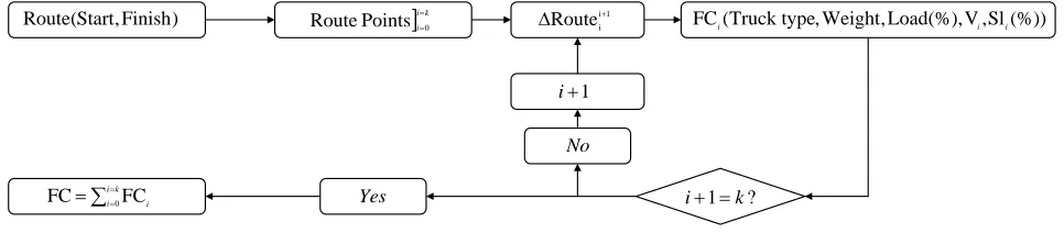
) Finish , Start (

Route



ik

i  0

Points

Route i1

i

Route



 

 ik i0FCi FC (%)) Sl , V (%), Load , Weight , Truck type (

FCi i i

1  i No ? 1 k i  Yes

Figure 1: General scheme of fuel consumption (FC) calculation for a particular route. Vi: Average velocity in section i; Average slope in sectioni.

physiographic characteristics of the area as well as the road infrastructure.

Under the conditions presented above, the main ob-jective of this study was to create an open software tool based on publicly accessible geographical data to assess biomass transportation fuel consumption, costs, and CO2 emissions. It is also an objective of this study to test the tool under realistic scenarios, namely the transportation of biomass for a pellets production plant located outside of the study area.

2 Methodology

2.1 General approach The method we developed is based on a set of variables that we considered as fun-damental to support a logistics model adjusted to any specific region. These include variables that are indepen-dent of spatial data and variables that require spatial data to be calculated.

In general terms, a logistics route is defined by a start-ing point (e.g., a forest industry for which biomass is destined) and an ending point (e.g., a forest where wood is collected). The location of each point is defined by its coordinates (latitude and longitude). In forestry, for one particular fixed starting point there is usually a large set of possible ending points in a region (e.g., all harvestable forest stands). An entire region must therefore be evalu-ated for each end point considered in the analysis. All regions have a set of potential points to define one route. Every starting point defines a set of coordinates for the truck travel to start. The ending points are set as a grid. An entire region is defined by the coordinates of two cor-ners of the grid: latmax, latmin, longmax, longmin. When a grid is defined by a matrix of (x, y) points, the coordi-nates of ending points are automatized (Supplementary Material A1).

For each ending point there is an optimal route (solved by OsmSharp.dll for a specific vehicle) to a starting point (this last is fixed) (Supplementary Ma-terial A2). Due to the large number of queries in-volved, the geographic data used is obtained from

OpenStreetMap©through downloading static databases from OpenStreetMap© Data Extracts [Available at: http://download.geofabrik.de/index.html]. The files extension are “pbf”, and the OsmSharp.dll has a specific instance to read this kind of file types us-ing the directives OsmSharp.Osm.PBF.Streams and OsmSharp.Routing.Osm.Interpreter to input the data in the system.

Each route is a set (0, 1, . . . , k) of geographic points denoted by (Route points]k₀), and each pair of consecu-tive points define a section (∆i+1_i Route). Each section has its properties and characteristics that affect fuel con-sumption (FC) calculation. Total fuel concon-sumption of a specific route is calculated as the summation of con-sumption in all sections from start to finish (Figure 1). 2.2 Fuel consumption calculation Fuel Consump-tion (FC) is directly related with i) Truck type, ii) Weight (truck + load), iii) Load proportion, iv) Truck speed, and v) Terrain slope [7] (see Supplementary Material B). For an individual transport from a starting point to an ending point, it can be assumed that truck type and weight are constant but speed and slope vary according to the spe-cific conditions in each of the sections of theA−B route where the truck is at a particular moment (Equation 1) [7].

F C =f(Truck type, Weight, Load %, V_i,Sli) (1)

Where:

F C= Fuel consumption (g/km),

Vi= Average velocity in sectioni(km/h),

Sli= Average slope in sectioni(%).

From the FC base calculation it is possible to obtain associated Fuel costs (Equation 2) and CO2 emissions (Equation 3).

Fcost =F C/(1000·DC)·di·P (2)

(4)

Table 1: Characteristics of different truck types considered in the tool for estimating fuel consumption and costs, and CO2 emissions of road transport in the Nordeste Transmontano region, Portugal.

Truck Type Weight (tonne) Weight (tonne) Weight (tonne) Load Width Length

category (Load 0%) (Load 100%) (tonne) (m) (m)

I

≤14 5 12 7 2.3 8

(Rigid Small) II

>14 10 28 18 2.3 12

(Rigid Big) III

≤32 12 26 14 2.4 12

(Articulated Small) IV

>32 20 45 25 2.5 16

(Articulated Big)

Fcost= Fuel cost (€),

FC= Fuel Consumption function (see Supplementary Material B),

DC = Fuel density (g/l), di= Length of section i(m),

P= Fuel Price (€/l).

ECO₂ =F C·C·_di (3)

WhereC= 3.16 is the Diesel-CO2 emission conversion factor [7].

2.3 Variables determination

2.3.1 Geographic data independent variables Truck type and load percentage are defined independently of geographic data. There are different kinds of trucks with different weights, lengths, and load characteristics. In this work we choose the more representative truck types used in forest biomass transportation in Portugal (Table 1).

The efficiency of using logistics resources is essential. For this reason, during transportation, trucks can travel completely filled (Load = 100%) in any of the routes. However, due to the particular characteristics of transport of wood it is possible that trucks travel empty (Load = 0%). Additionally, in some conditions it might be advantageous that trucks transport half of their capacity (Load = 50%).

2.3.2 Geographic data dependent variables A set of variables in the model requires geographic data to be derived from. In the following sections we describe how these variables are calculated.

Slope factor (Sli) The slope of a ∆Routei+1_i is

de-fined as the relative difference in elevation between points

iandi+1 divided by the distance between them

(Equa-tion 4).

Sli= (Elevi+1−Elevi)/di·100 (4)

Where:

Elevi and Elevi+1= Elevation of pointsi andi+1, respectively (m),

di= Horizontal length of section i(m).

The information included in static maps of OpenStreetMap© provided the latitude and longitude of all the points of an optimal route. Since elevation data is not part of this database, we used the Digital Elevation Model (DEM 30m Portugal WGS84, available in http://www.arcgis.com) in raster format for a matrix defined by location parameters similar to those used for the region (latmax, latmin, longmax, longmin). The ele-vation matrix data and the slope function calculation process is shown in Supplementary Material A3. Data is loaded in ASCII raster format. Number of rows and columns and resolution data are shown in the heading of the file.

Velocity Factor (Vi): The factor velocity is the

most complex variable in terms of calculation since it takes many factors into account. The velocity in a given section is determined by the minimum of three possible velocities (Equation 5): i) maximal legal, ii) maximal for the curve in terms of safety, and iii) velocity that the truck is able to achieve.

Vi=M in(Va, Vb, Vc) (5)

Where:

Va= Max legal velocity (km/h),

Vb = Max velocity for pass the curves with safety (km/h),

Vc= Estimation of velocity in section by Kinematic truck Model (km/h),

(5)

Max legal velocity (Va) OpenStreetMap© provides data containing Maximal legal velocity for each point of the optimal route, associated to each point by elements called tags. Max legal velocity data is obtained by two op-tions: i) “HighwayType” tag (this option is automatized according to the process described in Supplementary Ma-terial A4 where each “HighwayType” is associated to a generic maximal velocity (Decree-Law nº44/2005 of 23 February of Portugal) for each kind of road) and ii) “MaxSpeed” tag (this option does not appear in all cases, but when it does it is set as default for the max velocity). As in Supplementary Material A4, there is the pos-sibility of defining several values for the Coefficient of friction (µ) parameter for each possible road type. In this work, we consideredµ as a constant and equal to 0.5 [24].

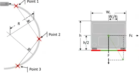
Maximum safe velocity (Vb) The maximum velocity

allowed for each road section was defined as equal to the force of the weight of the truck (F) and the centripetal force (Fc) in the basal range for a maximal safety range (Figure 2). The two forces are combined inVb (Equation

6) and in Supplementary Material A5.

Vb=p((Wi/4)/(h/2))·g·µ·R (6)

Where:

Vb = Maximum safe velocity,

Wi = The width of the truck, h = The height of the truck, g = Gravity force,

µ= Coefficient of friction of the road, R = The ratio of the curve.

Figure 2: Representation of the method to estimate the ratio of a curvature (R) between three consecutive points and the scheme of forces that affect the stability of a truck in a curve. The vector resulting from summing truck weight and centripetal forces determines if the truck can role or not. In this case the safety range falls into Wi/4 for each side of the truck.

The coefficient µ depends on the particular type of road under consideration but since data on this attribute is not provided by OSM it is not possible to establish this parameter. For that reason we assumedµconstant and equal to 0.5 [24].

Velocity in section (Vc): kinematic truck model

Truck speed at a particular instant in time is affected by various factors. In this study we considered only objective factors not taking into account subjective factors, such as experience or expertise of the driver, to simplify the process. We started from elementary physics according to which velocity at a certain instanti is equal to the initial velocity plus the acceleration in an instantiduring timet(Equation 7).

V ci=V ci−1+ai·t (7)

Where:

V ci−1= Initial velocity in section

ai= Instant acceleration,

t= Time.

Velocity depends essentially on instant acceleration (ai) at a particular time. To obtain this acceleration we used a kinematic application for truck movement [24, 25], as described in Equation 8.

ai= (Fi−Ri)/W (8)

Where:

Fi = Forces favorable to forward movement (N) at an instanti,

Ri= Resistance forces (N) at an instant i, W = Total mass of the truck (kg).

Acceleration is the difference between the forces that make the truck to advance (F) minus the reactive forces of the progression (R) [24] (Equation 9 and Equation 10).

F= min(F t, Fmax) (9)

Where:

F t= Tractive effort (N) which depends on i) the power of the truck, ii) the velocity at the time of calculation and iii) the efficiency in transmitting force,

Fmax = Maximum tractive force (N): which de-pends on i) the vehicle mass on tractive axle or axles and ii) friction coefficient (µ).

R=Ra+Rr+Rg (10)

(6)

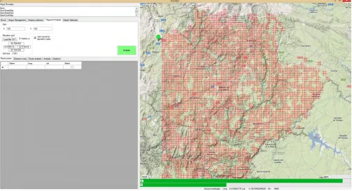
Figure 3: Main form of the application developed for estimating consumption, costs, and emissions of road transport in the Nordeste Transmontano region, Portugal.

Ra= Aerodynamic Resistance (N) which depends on i) truck frontal area, ii) truck speed, iii) truck drag coefficient, and iv) altitude coefficient,

Rr = Rolling resistance (N) which depends on i) total truck mass, ii) rolling coefficient, and iii) rolling resistance coefficients,

Rg= Slope resistance (N) which depends on i) total truck mass and ii) slope (%).

To obtain ai, Rakha et al. [24] used increments of time (∆t) to recalculate ai as a function of time. In this work we solved the same system but with increments of distance (∆d) because it is more operational in our model (Equation 11, Supplementary Material A6).

adi = (Fdi−Rdi)/W (11)

Where: di=d0+ ∆d

˙

v(di) ˙

x(di)

=

a(di)

v(di)

V ci=V ci−1+ai·t

xi=xi−1+Vi·t

2.4 Tool The pseudo code described in this paper can be compiled in different program languages. We developed an application form in C# language using

Visual Studio 2013 express (Microsoft Corporation) and the OsmSharp.dll (Figure 3) for applying the processes and methodology described above (see the main classes and procedures at Supplementary Material C). The in-terface of the application allows the user to define the area of analysis to be considered, the starting point and the ending grid points (x, y).

3 Application

We applied our tool in a real case scenario to analyse the efficiency and viability of road transport of resources with low value such as wood biomass. The particular objective of this application was to quantify costs, fuel consumption and CO2 emissions by truck type and fuel price in road transport of forest biomass from an entire region to a single destination (starting point): a pellets production plant located outside the study region. We wanted also to generate cost and CO2 emissions spatial surfaces for the study area to be used as criteria in a forest decision support system.

(7)

Table 2: Additional parameters for different truck types considered in the tool for estimating fuel consumption and costs, and CO2 emissions of road transport in the Nordeste Transmontano region, Portugal. “T. efficiency” is the coefficient of transmission efficiency; “A” is the truck frontal area (m2_{); “Cd” is the truck drag coefficient (%).}

Truck type Tractive axle Engine power T. efficiency A Cd

(%) (kW) (%) (m2₎ _(%)

I - Rigid small 67 186 89 6.8 70

II - Rigid large 8 246 89 6.8 70

III - Articulated small 31 335 89 10 70

IV - Articulated large 43.5 410 89 10.7 70

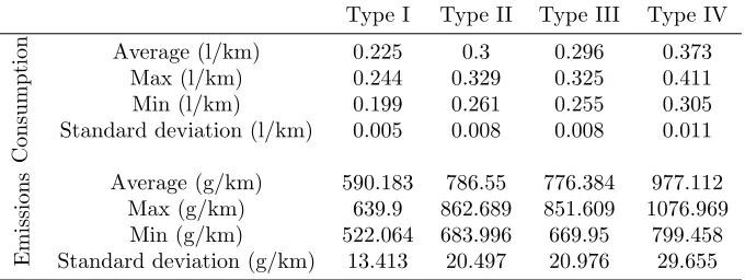
Table 3: General results of Fuel Consumption and CO2emissions for routes evaluated in the Nordeste Transmontano region, Portugal, by truck type analyzed.

Type I Type II Type III Type IV

Consumption

Average (l/km) 0.225 0.3 0.296 0.373

Max (l/km) 0.244 0.329 0.325 0.411

Min (l/km) 0.199 0.261 0.255 0.305

Standard deviation (l/km) 0.005 0.008 0.008 0.011

Emissions

Average (g/km) 590.183 786.55 776.384 977.112

Max (g/km) 639.9 862.689 851.609 1076.969

Min (g/km) 522.064 683.996 669.95 799.458

Standard deviation (g/km) 13.413 20.497 20.976 29.655

do Douro, Mirandela, and Macedo dos Cavaleiros). Total forest area in the region is 284,946 ha [5].

3.2 Inputs The tool was applied considering two types of trucks, rigid and articulated, and two size categories, small and big (Supplementary Material C).

The application was run under the following conditions (inputs):

• Region delimitation:

– Longmax= -7.4185806640. – Longmin= -6.1262890625. – Latmax= 42.02073285264. – Latmin= 40.96745587327.

• Grid size: x = 100, y = 100.

• Destination coordinates (starting point): – Endlat= 41.801519.

– Endlong= -7.452455.

• A run cycle consisted of a round trip from starting point (A) to ending point (B) with a load of 0% and return from ending point (B) to starting point (A) with load of 100%. In both cases (A-B and B-A) the optimal route was resolved independently, since road conditions and legal directions might change.

• Pick up sites (ending points) are stop places where trucks load wood; they exclude Motorways or in

Residential areas because wood loading would not be possible in these sites

• Additional truck parameters are shown in Table 2.

3.3 Results The application of the software tool under the conditions of the study area in the Northeast of Portugal allowed the estimation of a number of indicators of interest for the evaluation of transport of wood from any place in the region to a pellets industry located at the border of this area. The use of a 100 x 100 grid in the study region constrained by the destination coordinates returned 3,868 routes to potential collection points. Of these, only 3,107 satisfied the restriction of destination is a pick up site, since 761 fell in residential areas or motorways and are not suitable for wood loading.

Using only routes satisfying the criteria above, the application allowed extracting output data in tabular format concerning optimal distances, costs, and emissions, as well as maps representing the distribution of output simple and composite variables. The general results for fuel consumption and CO2 emissions according to the type of truck that can operate in the region are shown in Table 3.

(8)

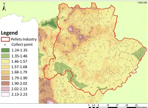
Figure 4: Fuel Consumption for truck type I (Rigid small) for the Nordeste Transmontano region, Portugal, in relation to a starting point corresponding to a wood pellets plant.

Figure 5: CO2emissions for truck type I (Rigid small) for the Nordeste Transmontano region, Portugal, in relation to a starting point corresponding to a wood pellets plant.

respectively, for truck type I). Maps for the remaining truck types (Fig. 7) are presented as supplementary ma-terial (Supplementary Mama-terial D).

The cost of transport depends directly on fuel price. Due to the high variability of diesel prices we analyzed the cost of consumption for different diesel prices in general for the region (Table 4). The average costs are repre-sentative of the entire region because they result from a large number of road types and different topography conditions in the region for the four truck types used in the simulations.

Estimates of distances can also be derived for each route and presented in absolute or relative terms thus providing additional information on transport efficiency

Table 4: General unitary cost per kilometer derived from fuel consumption data for four types of trucks in the Nordeste Transmontano region, Portugal.

Diesel price (€/l)

1.1 1.2 1.3 1.4

Average Type I 0.248 0.330 0.326 0.410

cost Type II 0.270 0.360 0.355 0.447

(€/km) Type III 0.293 0.390 0.385 0.484 Type IV 0.315 0.420 0.414 0.522

Table 5: Ratios of relation between routes from A to B (A-B) and B to A (B-A) with the beeline A-B in a sim-ple direction (Ratio A-B:Beeline and Ratio B-A:Beeline respectively) and from A to B to A with two times the beeline A–B (Ratio A-B-A:2Beeline) for the road system in the Nordeste Transmontano region, Portugal. A is the starting point (a wood pellets plant) and B are all collection points in the region. STD denotes standard deviation.

Ratio Ratio A-B:

Beeline

Ratio B-A: Beeline

Ratio A-B-A: 2Beeline

Average 1.6206 1.6235 1.6221

Max 2.2867 2.2909 2.2888

Min 1.2383 1.2289 1.2336

STD 0.1232 0.12 0.1212

and performance. In Table 5 and Figure 6, we present the average of the ratio between the road distance between starting point (A) and ending point (B) (both ways) and from point A to B and return, and the corresponding beeline distance (A and B).

4 Discussion

(9)

estab-Figure 6: Geographical data of Ratio (A-B-A: 2 Beeline) for the Nordeste Transmontano region in relation to a starting point corresponding to a wood pellets plant.

lish routes between points. The Open Source Data of OpenStreetMap© is constantly updated by community of volunteers revising periodically data which allows the periodic updating of the logistics indicators estimated by the software tool we developed. All inputs in the tool can be modified and it is possible to evaluate additional scenarios such as winter weather conditions, new types of vehicles and different velocity limits (for example for emergency vehicles).

In the case study of the Nordeste region, the applica-tion of the tool produced useful informaapplica-tion to support forest management decision-making. For example, it is possible from the outputs to locate sites for wood collec-tion with transportacollec-tion costs below a certain threshold established based on biomass prices at the destination (e.g., 30€/ton in Portugal). The same can be done for carbon dioxide. The results of the application of the tool can also support the definition and implementation of measures to minimize fuel consumption and thus CO2 emissions in forest logistics in the region. This can be achieved through selection of routes and areas where con-sumption was observed to be lower in relation to other routes or areas or where observed levels of consumption or emission were below a certain target value. In this regard, the tool can also be used to test the effects of changing not just physical aspects of the roads and the road network (pavement, design, etc.) but also vehicle technology (engine, tires, etc.) or human variables (driver experience) in fuel consumption and emissions.

The software tool we developed will produce informa-tion on logistics variables such as transport costs and CO2 emissions to be used as criteria in forest decision-making in the Nordeste Transmontano region with the purpose of optimizing the location of wood pellets plants

in the region, evaluating the economic viability of rout-ing and industry destinations, and evaluatrout-ing different alternatives in future road expansion.

5 Conclusions

In this work a software tool was developed to assess key determinants of forest logistics, in particular costs and CO2 emissions related to road transport. The tool uses different types of data (spatial and non-spatial) and has the flexibility to be adapted to the characteristics of any particular region. In the tool development, two empirical validated methodologies were used: the dy-namics model for maximum truck acceleration and the model of fuel consumption. It also combines the two creating a truck simulator applied to real surface spatial attributes. OpenStreetMap© is a reliable open source of geographical information, constantly maintained and updated and offering many capabilities to the user. The OpenStreetMap©offers the possibility of providing the statics maps that can be used in automatic routines using a large number of queries, like in our application. The tool and the development methodology proposed here can help to analyze spatial movement or resources taking into account different factors of particular regions such as road typology, truck types, topology, etc., to evaluate and map fuel consumption, costs and CO2, offering the possibility of taking these results into account in forest decision-making. The results of the application of our tool are important and very useful in providing spatial and numerical information that can be used in forest logistics in a given area to detect problems and to look for solutions to minimize costs and CO2 emissions, but there are many other possible applications.

Acknowledgments

This research was supported by the SIMWOOD project (Sustainable Innovative Mobilisation of Wood), EU FP7 Collaborative Project 2013-2017 Grant Agreement No. 613762. We thank Dr. Cesar Perez-Cruzado for his useful suggestions. We thank also two anonymous reviewers for valuable comments and suggestions on the manuscript.

References

[1] Abdulkarim, B., Kamberov, R., and Hay, G. J., 2014. Supporting urban energy efficiency with volunteered roof information and the Google Maps API. Remote Sensing 6 (10), 9691-9711. doi: 10.3390/rs6109691 [2] ANPEB, 2013. Relat´orio: A ind´ustria e mercado

(10)

[3] Azevedo, J. C., Castro, J. P., Tarelho, L., Escal-dante, E., Feliciano, M., 2011. Avalia¸cão do po-tencial de produ¸cão e utiliza¸cão sustentável de biomassa para energia no distrito de Bragan¸ca. Pro-cedings of 17ºCongresso da APDR. BRAGANÇ A and ZAMORA, 29 June 2011

[4] Azevedo, J. C., Ferreira, M. C., Nunes, L. F., Feli-ciano, M. 2016. What drives consumption of wood energy in the residential sector of small cities in Europe and how that can affect forest resources lo-cally? The case of Bragan¸ca, Portugal. International Forestry Review. 18(1):1-12.

[5] COS2007, 2007. Carta de Uso e Ocupa¸cão do Solo de Portugal Continental para 2007 (Direçcão-Geral do Território, DGT) Available online at http://www. dgterritorio.pt/cartografia e geodesia/cartografia/ cartografia tematica/cos/cos 2007/; last accessed Apr. 08, 2015.

[6] Ehrhardt, I., Seidel, H., Blobner, C., Schenk, E. H. M., 2013. Biomass logistics: the key of chal-lenge of minimizing supply costs. in Pethrick, R. A., Pearce, E. M., Zaikov, G. E., (eds.).Polymer Prod-ucts and Chemical Processes: Techniques, Analysis, and Applications. Apple Academic Press, Canada, pp. 257-295.

[7] EMEP/EEA, 2013. Air pollutant emission inventory guidebook 2013. Technical report No 12/2013. Copenhagen. Available online at: http://www.eea. europa.eu/publications/emep-eea-guidebook-2013; last accessed Apr. 08, 2015.

[8] Eriksson, L., Gustavsson. L., 2010. Costs, CO2-and primary energy balances of forest-fuel re-covery systems at different forest productivity. Biomass and Bioenergy 34 (5), 610-619. doi: 10.1016/j.biombioe.2010.01.003

[9] Faaij, A. P. C., 2006. Bio-energy in Europe: chang-ing technology choices. Energy Policy 34, 322-342. doi: 10.1016/j.enpol.2004.03.026

[10] Ferreira, J., Ferreira, M.E., 2011. Portugal: Pel-let report. ANPEB Portugal. Available online at: http://www.enplus-pellets.eu/wp-content/up-loads/2012/01/PT pellet report Jan2012.pdf; last accessed Apr. 08, 2015.

[11] Forghani, M., Delavar, M. A., 2014. Quality study of the OpenStreetMap dataset for Tehran. ISPRS International Journal of Geo-Information 3, 750-763. doi: 10.3390/ijgi3020750

[12] Fritz, S., McCallum, I., Schill, C., Perger, C., Grill-mayer, R., Achard, F., Kraxner, F., Obersteiner, M., 2009. Geo-Wiki.Org: The use of crowdsourcing to improve global land cover. Remote Sensing 1 (3), 345-354. doi: 10.3390/rs1030345

[13] Frisk, M., Göthe-Lundgren, M., Jörnsten, K., Rönnqvist, M., 2010. Cost allocation in collab-orative forest transportation. European Journal of Operational Research 205 (2), 448-458. doi: 10.1016/j.ejor.2010.01.015

[14] Frombo, F., Minciardia, R., Robba, M., Rosso, F., Sacile, R., 2009. Planning woody biomass lo-gistics for energy production: A strategic decision model. Biomass and Bioenergy 33, 372-383. doi: 10.1016/j.biombioe.2008.09.008

[15] Haklay, M., Weber, P., 2008. OpenStreetMap: User-generated street maps. IEEE Pervasive Computing 7 (4), 12-18. doi: 10.1109/MPRV.2008.80

[16] Haklay, M., 2010. How good is volunteered geo-graphical information? A comparative study of OpenStreetMap and Ordnance Survey datasets. En-vironment and Planning B: Planning and Design 37, 682-703. doi: 10.1068/b35097

[17] Han, S.K., Murphy, G. E., 2012. Solving a woody biomass truck scheduling problem for a transport company in Western Oregon, USA. Biomass and Bioenergy 44, 47-55. doi: 10.1016/j.biombioe.2012.04.015

[18] INE, 2014. Instituto Nacional de Estat´ıstica. Avail-able online at www.ine.pt; last accessed Apr. 08, 2015.)

[19] Kinoshita, T., Inoue, K., Iwao, K., Kagemoto, H., Yamagata, Y., 2009. A spatial evaluation of forest biomass usage using GIS. Applied Energy 86, 1-8. doi: 10.1016/j.apenergy.2008.03.017

[20] Luo, L., Wang, X., Guo, H., Liu, C., Liu, J., Li, L., Du, X., Qian G., 2014. Automated extraction of the archaeological tops of Qanat shafts from VHR imagery in Google Earth. Remote Sensing 6 (12), 11956-11976. doi: 10.3390/rs61211956

(11)

[23] Perpiña, C., Alfonso, D., Pérez-Navarro, A., Peñalvo, E., Vargas, C., Cárdenas R., 2009. Methodology based on Geographic Information Systems for biomass logistics and transport op-timisation. Renewable Energy 34, 555-565. doi: 10.1016/j.renene.2008.05.047

[24] Rakha, H., Lucic, I., Demarchi, S., Setti, J., Aerde, M., 2001. Vehicle Dynamics Model for Predicting Maximum Truck Acceleration Levels. Journal of Transportation Engineering 127 (5), 418 - 425. doi: 10.1061/(ASCE)0733-947X(2001)127:5(418) [25] Rakha, M., Lucic I., 2002. Variable power

ve-hicle dynamics model for estimating truck ac-celerations. Journal of Transportation Engineer-ing, 128 (5), 412-419. doi: 10.1061/(ASCE)0733-947X(2002)128:5(412)

[26] Ruiz, J.A., Ju´arez, M.C., Morales, M.P., Mu˜noz, P., Mend´ıvil M.A., 2013. Biomass logistics: Financial & environmental costs. Case study: 2 MW electrical power plants. Biomass and Bioenergy 56, 260-267. doi: 10.1016/j.biombioe.2013.05.014

[27] Santos, L., Coutinho-Rodrigues, J., Antunes, C. H., 2011. A web spatial decision support system for vehicle routing using Google Maps. Decision Support Systems 51 (1), 1-9. doi: 10.1016/j.dss.2010.11.008 [28] Schellekens, J., Brolsma, R.J., Dahm, R.J.,

Donchyts, G.V., Winsemius, H.C., 2014. Rapid setup of hydrological and hydraulic models using OpenStreetMap and the SRTM derived digital ele-vation model. Environmental Modelling & Software 61, 98-105. doi: 10.1016/j.envsoft.2014.07.006

[29] Sikkema, R., Junginger, M., Pichler, W., Hayes, S., Faaij, A.P.C., 2010. The international logistics of wood pellets for heating and power production in Europe: Costs, energy-input and greenhouse gas bal-ances of pellet consumption in Italy, Sweden and the Netherlands. Biofuels, Bioproducts and Biorefining 2 (4), 132-153. doi: 10.1002/bbb.208

[30] Steiniger, S., Hay, G. J., 2009. Free and open source geographic information tools for landscape ecology. Ecological Informatics 4 (4), 183-195. doi: 10.1016/j.ecoinf.2009.07.004

[31] Viana, H., Cohen, W.B., Lopes, D., Aranha, J., 2010. Assessment of forest biomass for use as energy. GIS-Based analysis of geographical avail-ability and locations of wood-fired power plants in Portugal. Applied Energy 8 (87), 2551-2560. doi:10.1016/j.apenergy.2010.02.007

[32] Wolfsmayr, U.J., Rauch, P. (2014) The primary for-est fuel supply chain: A literature review. Biomass and Bioenergy 60: 203–221

[33] Yemshanov, D., McKenney, D. W., Fraleigh, S., Mc-Conkey, B., Huffman,, T., Smith S., 2014. Cost estimates of post harvest forest biomass supply for Canada. Biomass and Bioenergy 69, 80-94. doi: 10.1016/j.biombioe.2014.07.002

(12)

A

Supplementary Material: Pseudo codes

A1 : Pseudo c o d e t o a u t o m a t i z e c o o r d i n a t e s o f e n d i n g p o i n t s using a g r i d i n a d e l i m i t e d r e g i o n .

Using : OSMSharp P r o c e d u r e : Region

I n p u t : C o o r d i n a t e Longmin , Latmin Longmax Latmax For (i n t i = 0 ; i <= a ; i ++)

For (i n t j = 0 ; j <= b ; j ++)

e n d l o n = ( Longmin ) + ( Math . Abs ( Longmin − Longmax ) / a ) ∗ i ; e n d l a t = ( Latmin ) + ( ( Latmin − Latmax ) / b ) ∗ j ;

s t a r t = new PointLatLng ( s t a r l a t , s t a r l o n g ) ; end = new PointLatLng ( e n d l a t , e n d l o n g ) ; End f o r

End f o r

Return : PointLatLng s t a r t End p r o c e d u r e : Region

A2 : Pseudo c o d e f o r r o u t e o p t i m i z a t i o n between two c o o r d i n a t e s using OsmSharp . Osm . PBF . Streams ;

using OsmSharp . Routing ;

using OsmSharp . Routing . Osm . I n t e r p r e t e r ; P r o c e d u r e : OptimalRoute

I n p u t : C o o r d i n a t e s t a r t L a t , s t a r t L n g , end Lat , end Lng v a r r e s o l v e d 1 = r o u t e r . R e s o l v e ( V e h i c l e . BigTruck , new OsmSharp . Math . Geo . G eoCo ordina te ( s t a r t L a t , s t a r t L n g ) ) ; v a r r e s o l v e d 2 = r o u t e r . R e s o l v e ( V e h i c l e . BigTruck , new OsmSharp . Math . Geo . G eoCo ordina te ( end Lat , end Lng ) ) ;

// c a l c u l a t e r o u t e .

v a r r o u t e = r o u t e r . C a l c u l a t e ( V e h i c l e . BigTruck , r e s o l v e d 1 , r e s o l v e d 2 ) ; Return r o u t e ;

End p r o c e d u r e

A3 : Pseudo c o d e f o r s l o p e e s t i m a t i o n between two p o i n t s using a s p e c i f i c DEM i n ASCII f o r m a t .

Using : OSMSharp P r o c e d u r e : Region

I n p u t : C o o r d i n a t e Longmin , Latmin Longmax Latmax For (i n t i = 0 ; i <= a ; i ++)

For (i n t j = 0 ; j <= b ; j ++)

e n d l o n = ( Longmin ) + ( Math . Abs ( Longmin − Longmax ) / a ) ∗ i ; e n d l a t = ( Latmin ) + ( ( Latmin − Latmax ) / b ) ∗ j ;

s t a r t = new PointLatLng ( s t a r l a t , s t a r l o n g ) ; end = new PointLatLng ( e n d l a t , e n d l o n g ) ; End f o r

End f o r

Return : PointLatLng s t a r t End p r o c e d u r e : Region

A4 : Pseudo c o d e f o r t h e e s t a b l i s h m e n t o f l e g a l v e l o c i t y using t h e OpenStreetMap Data ” HighwatType ” t a g .

(13)

i f ( HighwayType == ” motorway ” ) −> Va = 1 0 0 ; } i f ( HighwayType == ” t r u n k ” ) −> Va = 8 0 ; } i f ( HighwayType == ” p r i m a r y ” ) −> Va = 8 0 ; } i f ( HighwayType == ” s e c o n d a r y ” ) −> Va = 7 0 ; } i f ( HighwayType == ” t e r t i a r y ” ) −> Va = 7 0 ; } i f ( HighwayType == ” u n c l a s s i f i e d ” ) −> Va = 8 0 ; } i f ( HighwayType == ” r e s i d e n t i a l ” ) −> Va = 4 0 ; } i f ( HighwayType == ” s e r v i c e ” ) −> Va = 3 0 ; }

i f ( HighwayType == ” m o t o r w a y l i n k ” ) −> Va = 6 0 ; } i f ( HighwayType == ” t r u n k l i n k ” ) −> Va = 6 0 ; } i f ( HighwayType == ” p r i m a r y l i n k ” ) −> Va = 5 0 ; } i f ( HighwayType == ” s e c o n d a r y l i n k ” ) −> Va = 5 0 ; } i f ( HighwayType == ” t e r t i a r y l i n k ” ) −>Va = 5 0 ; } i f ( HighwayType == ” l i v i n g s t r e e t ”)−>Va = 3 0 ; } i f ( HighwayType == ” p e d e s t r i a n ”)−>Va = 2 0 ; } i f ( HighwayType == ” t r a c k ”)−> Va = 2 0 ;

Return Va ;

End p r o c e d u r e : M a x L e g a l V e l o c i t y

A5 : Pseudo c o d e f o r t h e c a l c u l a t i o n o f t h e r a t i o o f c u r v a t u r e between two c o o r d i n a t e s .

P r o c e d u r e : C u r v a t u r e

I n p u t : double X1 , double Y1 , double X2 , double Y2 , double X3 , double Y3 double R a t i o ;

double a = Math . S q r t ( Math . Pow( X1 − X2 , 2 ) + Math . Pow( Y1 − Y2 , 2 ) ) ∗ 1 0 0 ; double b = Math . S q r t ( Math . Pow( X2 − X3 , 2 ) + Math . Pow( Y2 − Y3 , 2 ) ) ∗ 1 0 0 ; double c = Math . S q r t ( Math . Pow( X3 − X1 , 2 ) + Math . Pow( Y3 − Y1 , 2 ) ) ∗ 1 0 0 ; double d e n R a t i o = ( Math . S i n ( Math . Acos ( ( Math . Pow( a , 2 ) − Math . Pow( b , 2 ) − Math . Pow( c , 2 ) ) / (−2 ∗ b ∗ c ) ) ) ) ∗ 2 ;

Return R a t i o ∗ 1000 End p r o c e d u r e : C u r v a t u r e

A6 : Pseudo c o d e t o e s t i m a t e t h e v e l o c i t y o f a t r u c k between two p o i n t s . P r o c e d u r e : Vc

I n p u t : double v e l o c i t y , double d i s t a n c e , double w e i g ht , double mu, double s l o p e , double e l e v a t i o n , double power

For (i n t i = 0 ; i <= d i s t a n c e∗1 0 0 0 ; i ++)

// C a l c u l a t e F

Double Mta ; // = D e f i n e p a r a m e t e r Mta ;

double F = 9 . 8 0 6 6 ∗ w e i g h t ∗ Mta ∗ mu ;

// C a l c u l a t e Ft

double Ft = 3600 ∗ 0 . 8 9 ∗ ( power / v e l o c i t y ) ;

// C a l c u l a t e Ra

double c1 = 0 . 0 4 7 2 8 5 ; // i s c o n s t a n t ;

double Cd = // = D e f i n e p a r a m e t e r Cd ; ;

double Ch = 1 − 0 . 0 0 0 0 8 5 ∗ e l e v a t i o n ; double A;// = D e f i n e p a r a m e t e r A;

double Ra = c1 ∗ Cd ∗ Ch ∗ A ∗ Math . Pow( v e l o c i t y , 2 ) ;

// C a l c u l a t e Rr

double Cr ; // = D e f i n e p a r a m e t e r Cr ;

double C2 ; // = D e f i n e p a r a m e t e r C2 ;

double C3 ; // = D e f i n e p a r a m e t e r C3 ;

double Rr = 9 . 8 0 6 6 ∗ Cr ∗ ( C2 ∗ v e l o c i t y + C3 ) ∗ w e i g t h / 1 0 0 0 ;

(14)

double Rg = 9 . 8 0 6 6 ∗ w e i g h t ∗ s l o p e / 1 0 0 ;

// C a l c u l a t e R

double R = Ra + Rr + Rg ;

double a = ( Math . Min (F , Ft ) − R) / w e i g h t ; double t = ( d i s t a n c e / 1 0 0 0 ) / v e l o c i t y ; Vci = Vci−1 + a ∗ t ;

End f o r Return Vci

End p r o c e d u r e : Vc

B

Supplementary Material — Equations applied in fuel consumption calculation:

FC (Truck type, Weight Load percentage, Velocity, Slope)

Font: EMEP/EEA (2013) Table B: Equations applied in fuel consumption calculation: FC (Truck type, Weight Load percentage, Velocity, Slope).

T. type % slope % load Eq. Type1 a b c d e

I -6 0 Eq. A 664.55823 0.9570022 -0.5134748 -

-I -6 50 Eq. B -7.9777611 182.13264 5.5153746 2.0975186 -0.0089466

I -6 100 Eq. B -7.5394195 166.29979 5.8176705 2.1677622 -0.009613

I -4 0 Eq. C 11.28247 -15.5865 -2.0177201 -

-I -4 50 Eq. C 12.056496 -19.532977 -2.2067022 -

-I -4 100 Eq. D -0.0008254 0.1542265 -9.9851294 237.76994

-I -2 0 Eq. D 2917.7595 1.0125629 -1.1430934 -

-I -2 50 Eq. C 7.9292672 -2.478343 -0.9694032 -

-I -2 100 Eq. D -0.0010026 0.1876354 -12.360846 332.17662

-I 0 0 Eq. A 2028.4551 1.0146246 -0.898327 -

-I 0 50 Eq. A 1691.0673 1.0107097 -0.7638133 -

-I 0 100 Eq. A 1478.6155 1.0074281 -0.6540388 -

-I 2 0 Eq. A 1443.0554 1.0126787 -0.6664953 -

-I 2 50 Eq. A 1285.8385 1.0099298 -0.5414106 -

-I 2 100 Eq. A 1216.0173 1.0077448 -0.4507751 -

-I 4 0 Eq. A 1211.9379 1.01057 -0.5063448 -

-I 4 50 Eq. A 1063.3692 1.0070366 -0.3570552 -

-I 4 100 Eq. A 1048.9866 1.0048163 -0.2719746 -

-I 6 0 Eq. A 1029.7032 1.0076371 -0.3587513 -

-I 6 50 Eq. E 1488.0338 -0.684967 215.96762 0.1535674

-I 6 100 Eq. D -0.0024109 0.3176589 -14.466683 842.45479

-II -6 0 Eq. C 13.758599 -23.442671 -2.6962432 -

-II -6 50 Eq. B -14.55865 311.60501 4.6595269 1.8456395 -0.0060372

II -6 100 Eq. B -12.621964 245.52814 5.6714483 2.0881829 -0.0084357

II -4 0 Eq. A 1188.5325 0.9689277 -0.5159119 -

-II -4 50 Eq. A 759.80631 0.9621383 -0.3099059 -

-II -4 100 Eq. D -0.0011814 0.2244267 -14.955974 368.97118

-II -2 0 Eq. C 8.2647891 -1.4857645 -0.9654162 -

-II -2 50 Eq. D -0.001678 0.305809 -19.767193 518.63079

-II -2 100 Eq. D -0.001599 0.2939372 -19.698191 546.27395

-II 0 0 Eq. A 2509.1997 1.0081738 -0.7632624 -

-II 0 50 Eq. A 2072.2285 1.004001 -0.6068544 -

(15)

-II 2 0 Eq. A 2119.256 1.0092279 -0.6106017 -

-II 2 50 Eq. A 1915.8423 1.0068375 -0.4698263 -

-II 2 100 Eq. A 1875.3849 1.004855 -0.3764674 -

-II 4 0 Eq. A 1945.7298 1.0088558 -0.4935859 -

-II 4 50 Eq. A 1709.1108 1.0052248 -0.316049 -

-II 4 100 Eq. A 1777.3794 1.0032778 -0.2336836 -

-II 6 0 Eq. E 177.107 0.2371867 3411.2551 -0.8258885

-II 6 50 Eq. A 1767.1442 1.0042966 -0.2379125 -

-II 6 100 Eq. D -0.0060042 0.7078024 -29.340175 1576.6602

-III -6 0 Eq. C 14.105519 -25.449992 -2.8173741 -

-III -6 50 Eq. B -10.624079 228.76887 5.8694875 2.1813923 -0.0099616

III -6 100 Eq. B -9.5945152 193.8603 6.7541126 2.3960349 -0.0120616

III -4 0 Eq. A 930.32642 0.9654672 -0.4465249 -

-III -4 50 Eq. A 594.30572 0.9595132 -0.238592 -

-III -4 100 Eq. D -0.0010874 0.2067291 -13.803647 341.58295

-III -2 0 Eq. C 9.0051657 -5.1946817 -1.1809174 -

-III -2 50 Eq. D -0.0015042 0.2759418 -18.04247 478.22576

-III -2 100 Eq. D -0.0014681 0.2706602 -18.290058 512.42884

-III 0 0 Eq. A 2478.5936 1.008829 -0.7890916 -

-III 0 50 Eq. A 1915.303 1.0035637 -0.5944679 -

-III 0 100 Eq. D -0.0013695 0.2718437 -19.157568 713.75302

-III 2 0 Eq. A 1975.4006 1.0093608 -0.603163 -

-III 2 50 Eq. A 1737.9492 1.0062261 -0.4405978 -

-III 2 100 Eq. D -0.001166 0.2427845 -16.949773 924.93652

-III 4 0 Eq. A 1695.3459 1.0081499 -0.4508975 -

-III 4 50 Eq. A 1521.9599 1.0041984 -0.272479 -

-III 4 100 Eq. D -0.0023663 0.354921 -18.952371 1201.16

-III 6 0 Eq. E 233.33757 0.1807236 2927.9411 -0.830322

-III 6 50 Eq. D -0.0026727 0.3861257 -19.093328 1198.0769

-III 6 100 Eq. D -0.0054854 0.604789 -25.007723 1534.0413

-IV -6 0 Eq. C 14.286351 -24.322312 -2.8154203 -

-IV -6 50 Eq. C 14.848828 -28.388124 -2.9396773 -

-IV -6 100 Eq. C 15.215195 -31.557912 -2.9966331 -

-IV -4 0 Eq. A 1417.7307 0.9661542 -0.5186673 -

-IV -4 50 Eq. A 701.9861 0.9569389 -0.1810194 -

-IV -4 100 Eq. D -0.0014343 0.2738379 -18.471373 464.15915

-IV -2 0 Eq. C 9.8096307 -7.3464493 -1.343481 -

-IV -2 50 Eq. D -0.001959 0.3585134 -23.642726 634.5643

-IV -2 100 Eq. D -0.0018715 0.3473962 -24.201914 708.18899

-IV 0 0 Eq. A 3135.9922 1.0078183 -0.7952219 -

-IV 0 50 Eq. A 2183.5942 1.0005483 -0.5099369 -

-IV 0 100 Eq. D -0.0017824 0.350877 -25.570092 1017.3698

-IV 2 0 Eq. A 2561.6186 1.009353 -0.6253269 -

-IV 2 50 Eq. A 2148.8362 1.0047625 -0.3851695 -

-IV 2 100 Eq. A 2174.1709 1.0016168 -0.264482 -

-IV 4 0 Eq. A 2178.9225 1.0082996 -0.4715468 -

-IV 4 50 Eq. C 7.0045674 2.2388545 -0.0537346 -

-IV 4 100 Eq. D -0.0067764 0.752455 -32.691171 1870.6569

-IV 6 0 Eq. E 4097.538 -0.8883607 296.50747 0.1697847

-IV 6 50 Eq. D -0.0089576 0.9834534 -37.968038 1805.087

-IV 6 100 Eq. D -0.0357516 2.8599895 -81.501354 2682.0619

-1_{Eq. Type: Eq. A:}_{F C}₌_a_·_bV

·(Vc_{). Eq. B:}_{F C}₌_a_{+ (}_b_{/ (1 + exp (-1}_·_c₊_d_·_{ln(V) +}_e_·_{V))). Eq. C:}_{F C}_{= exp (}_a₊_b/_{V + c}_·_{ln (V)).}

(16)

C

Supplementary Material: Code source of the main procedures of the

applica-tion in C# language

// C l a s s e s :

c l a s s Truck {

public double EnginePower { g e t ; s e t ;}

public double T r a n s m i s i o n E f i c i e n c y { g e t ; s e t ; } public i n t Type{ g e t ; s e t ; }

public double P e r c T r a n s m i s i o n A x l e { g e t ; s e t ;} public double AreaCabin { g e t ; s e t ;}

public double TotalWeigth { g e t ; s e t ;}

// C o n s t a n t e q u a l s t o 0 . 0 4 7 2 8 5

public double c1 { g e t ; s e t ;}

//Cd : Truck d r a g c o e f f i c i e n t

public double Cd { g e t ; s e t ;}

//Cr : r o l l i n g c o e f f i c i e n t

public double Cr { g e t ; s e t ;}

//C1 and C2 : r o l l i n g r e s i s t a n c e c o e f f i c i e n t

public double C2 { g e t ; s e t ;} public double C3 { g e t ; s e t ;} }

// P r o c e d u r e s :

// Truck A c e l e r a t i o n

public s t a t i c double A c e l e r a t e d S p e e d (double I n i t i a l S p e e d , double d i s t a n c e , Truck t r u c k , double mu, double s l o p e , double e l e v a t i o n )

{

f o r (i n t i = 0 ; i <= d i s t a n c e∗1 0 0 ; i ++) {

double F = 9 . 8 0 6 6 ∗ t r u c k . TotalWeigth ∗ t r u c k . P e r c T r a n s m i s i o n A x l e ∗ mu ;

double Ft = 3600 ∗ t r u c k . T r a n s m i s i o n E f i c i e n c y ∗ ( t r u c k . EnginePower / I n i t i a l S p e e d ) ; double Ch = 1 − 0 . 0 0 0 0 8 5 ∗ e l e v a t i o n ;

double Ra = t r u c k . c1 ∗ t r u c k . Cd ∗ t r u c k . Ch ∗ t r u c k . AreaCabin ∗ Math . Pow( I n i t i a l S p e e d , 2 ) ;

double Rr = 9 . 8 0 6 6 ∗ t r u c k . Cr ∗ ( t r u c k . C2 ∗ I n i t i a l S p e e d + t r u c k . C3 ) ∗ t r u c k . TotalWeigth / 1 0 0 0 ;

double RG = 9 . 8 0 6 6 ∗ t r u c k . TotalWeigth ∗ s l o p e / 1 0 0 ; double R = Ra + Rr + RG;

double a = ( Math . Min (F , Ft ) − R) / t r u c k . TotalWeigth ; double t = ( d i s t a n c e / 1 0 0 0 ) / I n i t i a l S p e e d ;

I n i t i a l S p e e d = I n i t i a l S p e e d + a ∗ t ; }

return I n i t i a l S p e e d ; }

// C u r v a t u r e

// Needed t h r e e c o n s e c u t i v e p o i n t s (X1 , Y1 ) , (X2 , Y2) and (X3 , Y3)

public s t a t i c Double C u r v a t u r e (double X1 , double Y1 , double X2 , double Y2 , double X3 , double Y3 )

{

(17)

double a = Math . S q r t ( Math . Pow( X1 − X2 , 2 ) + Math . Pow( Y1 − Y2 , 2 ) ) ∗ 1 0 0 ; double b = Math . S q r t ( Math . Pow( X2 − X3 , 2 ) + Math . Pow( Y2 − Y3 , 2 ) ) ∗ 1 0 0 ; double c = Math . S q r t ( Math . Pow( X3 − X1 , 2 ) + Math . Pow( Y3 − Y1 , 2 ) ) ∗ 1 0 0 ; double d e n R a t i o = ( Math . S i n ( Math . Acos ( ( Math . Pow( a , 2 ) − Math . Pow( b , 2 ) − Math . Pow( c , 2 ) ) / (−2 ∗ b ∗ c ) ) ) ) ∗ 2 ;

i f ( d e n R a t i o < 0 . 0 0 0 1 | | double. IsNaN ( d e n R a t i o ) ) {

R a t i o = 0 ; }

e l s e {

R a t i o = a / ( Math . S i n ( Math . Acos ( ( Math . Pow( a , 2 ) − Math . Pow( b , 2 ) − Math . Pow( c , 2 ) ) / (−2 ∗ b ∗ c ) ) ) ) ∗ 2 ;

}

return R a t i o ∗ 1 0 0 0 ; }

// Load t h e e l e v a t i o n u s i n g a ASCII DEM

public s t a t i c double[ , ] e l e v a t i o n M a t r i x (double maxX , double minX , d o u b l e maxY , double minY , double s i z e , s t r i n g f i l e p a t h )

{

i n t c o u n t e r = 0 ; i n t c o u n t e r 2 = 0 ; s t r i n g l i n e ;

i n t x i d = Convert . ToInt32 ( ( maxX − minX ) / s i z e ) ; i n t y i d = Convert . ToInt32 ( ( maxY − minY ) / s i z e ) ; double[ , ] mT = new double[ xid , y i d ] ;

// Read t h e f i l e and d i s p l a y i t l i n e by l i n e .

System . IO . StreamReader f i l e =

new System . IO . StreamReader ( f i l e p a t h ) ; while ( ( l i n e = f i l e . ReadLine ( ) ) != n u l l ) {

i f ( c o u n t e r > 5 ) {

s t r i n g b = ” ” ; b = l i n e ;

f o r (i n t i = 0 ; i < b . S p l i t (new Char [ ] { ’ , ’ , ’ ’ }) . Count ( )−1 ; i ++) {

mT[ i , c o u n t e r 2 ] = Convert . ToDouble ( b . S p l i t (new Char [ ] { ’ , ’ , ’ ’ }) . ElementAt ( i ) . T o S t r i n g ( ) ) ;

}

c o u n t e r 2 ++; }

c o u n t e r ++; }

f i l e . C l o s e ( ) ; return mT; }

// S l o p e c l a s s e s

public s t a t i c i n t s l o p e c l a s s (double s l o p e ) {

(18)

i f ( s l o p e < −6) { s l o p e c a s e = −6; } e l s e i f ( s l o p e < −4) { s l o p e c a s e = −4; } e l s e i f ( s l o p e < −2) { s l o p e c a s e = −2; } e l s e i f ( s l o p e < 0 ) { s l o p e c a s e = 0 ; } e l s e i f ( s l o p e < 2 ) { s l o p e c a s e = 0 ; } e l s e i f ( s l o p e < 4 ) { s l o p e c a s e = 2 ; } e l s e i f ( s l o p e < 6 ) { s l o p e c a s e = 4 ; } e l s e { s l o p e c a s e = 6 ; }

return s l o p e c a s e ; }

// E s t a b l i s h m e n t o f max l e g a l v e l o c i t y c l a s s e s

public s t a t i c Double maxVel ( s t r i n g HighwayType ) {

i f ( HighwayType == ” motorway ” ) { return 1 0 0 ; } i f ( HighwayType == ” t r u n k ” ) { return 8 0 ; } i f ( HighwayType == ” p r i m a r y ” ) { return 8 0 ; } i f ( HighwayType == ” s e c o n d a r y ” ) { return 7 0 ; } i f ( HighwayType == ” t e r t i a r y ” ) { return 7 0 ; } i f ( HighwayType == ” u n c l a s s i f i e d ” ) { return 8 0 ; } i f ( HighwayType == ” r e s i d e n t i a l ” ) { return 4 0 ; } i f ( HighwayType == ” s e r v i c e ” ) { return 3 0 ; }