https://doi.org/10.26637/MJM0S01/07
A two storage inventory model with variable demand
and time dependent deterioration rate and with
partial backlogging
Richi Singh
1*, Ashok Kumar
2and Dharmendra Yadav
3Abstract
In this paper an inventory model is developed for single deteriorating items, partially backlogged shortages under two storehouses (first is owned and second is rented warehouse). The deterioration rate has been considered here to be time dependent. The demand rate of the item depends on (1) time; (2) selling price; and (3) the frequency of advertisement. The stocks of first warehouse are filled from second warehouse by using continuous release pattern. Here different cases and sub-cases are assumed according to the stock level at initial and reorder points, with respect to the relative size of storing capacities of storehouses. The proposed inventory model is formulated for each sub-case as non linear constrained mixed integer optimization problem. Here GRG technique is used to solve the problem. Also a numerical example is presented to demonstrate the proposed model.
Keywords
Two-storehouse inventory; Variable deterioration rate; Variable demand rate; Partial backlogging.
1Research Scholar, Meerut College Meerut, Uttar Pradesh, India.
2Meerut College, Meerut, Uttar Pradesh, India.
3Vardhman College, Bijnore, Uttar Pradesh, India.
*Corresponding author:1[email protected];2[email protected];3[email protected]
Article History: Received24December2017; Accepted21January2018 c2018 MJM.
Contents
1 Introduction. . . 35
2 Notations and assumptions. . . 36
3 Mathematical formulation. . . 36
4 Numerical illustration. . . 39
5 Conclusions. . . 39
References. . . 39
1. Introduction
Hartely (1976) firstly worked on inventory models assum-ing two storehouses and constant demand rate. Decayassum-ing items are the items that happen to spoil, damage, lost of its marginal value, and so on through time. The deterioration of products in inventory is an actual characteristic that is neces-sary to study its effect on inventory. Yang (2004) and Hsieh et al., (2008) analysed inventory models for decaying items assuming two storehouses. Xu et al., (2017) analysed two storehouses inventory model with different policies of
backlogging and time dependent (linear) deterioration rate. In Section 2 the notations and assumptions of the model are shown. In section 3 mathematical formulations of different cases with sub-cases are discussed. In Section 4, a numerical example and optimal solution is presented. Section 5 gives concluding remark and scope for the future research.
2. Notations and assumptions
The mathematical model rest on the following assump-tions:
(1) The rate of replenishment is taken infinite.
(2) Lead time is taken constant.
(3) The rate of demand rate is taken asD(N,p,t) =Nγ(a− bp+ct),a,b,c,γ>0.
(4) Extent of inventory scheduling is taken infinite.
(5) The entire lot size is supplied in one batch.
(6) Both the warehouses are of finite storing capacities.
(7) The time gap in selling from first storehouse (OW) and occupying the space by the units of second storehouse (RW) is not significant.
(8) Backlogging rate is taken as[1+δ(T−t)]−1, whereδ >0.
The mathematical model rest on the following notations:
I(t): Inventory level during timet.
H1: Storing capacity of first storehouse (OW). H2: Storing capacity of second storehouse (RW). S: Highest stock level (initially)
L1: An inventory system having a single storing facility. L2: An inventory system having two storing facilities. C1: Holding cost of 1 unit in 1 unit of time at first storehouse (OW).
C10 (C10 >C1): Holding cost of 1 unit in 1 unit of time at second storehouse (RW).
C2: Shortage cost of 1 unit in 1 unit of time. C3: Purchase cost of 1 unit of item.
C4: Transportation cost 1 unit of item.
θOW(t):(=a1+b1t): Rate of decay in OW, wherea1is scale parameter and 0<b1<1.
θRW(t):(=a2+b2t): Rate of decay in RW, wherea2is scale parameter and 0<b2<1.
R: Reorder point.
A1: Replenishment cost/ordering cost per replenishment for L1system.
A2: Replenishment cost/ordering cost per replenishment for L2system.
m(>1): The mark up rate.
p: Selling price per unit of item, which is taken asp=mCp.
N: Rate of recurrence of advertisement. A: Advertisement cost per advertisement. T: The duration of cycle.
3. Mathematical formulation
According to the storage capacities of both store houses and highest stock level, two cases arise:
Case 1:H1<S≤H1+H2(L2system)
Case 2:S≤H1(L1system)
According to the reorder point of stock level four sub-cases may arise:
Sub-case 3.1:H1<S≤H1+H2andR<0 Sub-case 3.2:H1<S≤H1+H2andR>0 Sub-case 3.3:S≤H1andR<0
Sub-case 3.4:S≤H1andR>0 The Sub-case 3.1 is explained as follows
Sub-case 3.1:H1<S≤H1+H2andR<0
Figure 1
Inventory levelIr(t)at second storehouse (RW) is pre-sented by the following equations
dIr(t)
dt + (a2+b2t)Ir(t) =−D(t), 0≤t≤t1 (1) s. t.
Ir(t1) =0, (2)
Ir(t) =S−H1att=0 (3)
Using equation (2), the solution of equation (1) is as follows
Ir(t) =−Nγ(t−t1)
(a−bp) +{(a−bp)a2+c}
t+t
1 2
e−(a2t+b2t 2
2) (4)
Using equation (3),
S=H1+Nγt1
(a−bp) +{(a−bp)a2+c} t1 2
(5)
In first storehouse (OW) the inventory levelIo(t)during[0,T] is presented as
dIo(t)
dt + (a1+b1t)Io(t) =0, 0≤t<t1 (6) dIo(t)
dt + (a1+b1t)Io(t) =−D(t), t1≤t≤t2 (7) dIo(t)
dt =−
D(t)
1+δ(T−t), t2<t≤T (8)
s. t.
Io(t) =H1 att=0, (9)
Io(t) =0 att=t2 (10)
and
Io(t) =−R att=T. (11)
Using the continuity ofIo(t)att1andt2and above conditions the solutions of the equations are as follows
Io(t) =H1e−(a1+b1 t2
2), 0≤t<t
1 (12)
Io(t) =−Nγ(T−t2)
(a−bp) +{(a−bp)a1+c}
t+t2 2
e−(a1t+b1t 2
2), t1≤t≤t2 (13)
Io(t) =
Nγ δ
a−bp+c
T+1 δ
log|1+δ(T−t)| −c(T−t)
−R, t2<t≤T
(14)
and, we have
H1=−Nγ(t1−t2)
(a−bp) +{(a−bp)a1+c}
t
1+t2 2
(15)
The above equation reduces toAt22+Bt2−C=0, whereA= Nγ{(a−bp)a
1+c},B=2Nγ(a−bp),C=2W1+2Nγ+ (a− bp)t1+Nγt12{(a1−bp)a1+c}gives the solution
t2=−B+
√
B2+4AB
2A (16)
Using equations (13) and (14)
R=N γ
δ
a−bp+c
T+1 δ
log|1+δ(T−t2)| −c(T−t2)
(17)
The Inventory carrying units in second storehouse (RW)=
Rt1
0 Ir(t)dt
=N γ
24t 2
1{4(a−bp)(3−a2t1) +t1(8−3a2t1)}. (18)
The Inventory carrying units in first storehouse
(OW) =
Z t2
0 Io(t)dt
=H1(t1−a1 t12
2) + Nγ
6 (a−bp)(t1−t2) 2
{3−a1(2t1+t2)} − Nγ
12{(a−bp)a1+c}(t1−t2) 2
{3a1t12−t2(8−3a1t2)−t1(4−6a1t2)}. (19)
The total shortage cost
=C2
Z T
t2
[−I0(t)]dt
=−C2
Nγ δ
a−bp+c
T+1 δ
1
dlog|1+δ(T−t2)|{1+δ(T−t2)} −(T−t)}
−c(t−t2) 2
2
−R(T−t2)
(20)
The total transportation cost
=Ct
Z t1
0
D(N,pt)dt=CtNγ
(a−bp)t1+ c 2t 2 1 (21)
Now total profit(P=total sales revenue – total cost of the system
P(N,t1,T)
=p
Nγ
(a−bp)t2+ c 2t
2 2
+|R|
−C3(S+|R|)−(R1+R2)
−C1
H1(t1−a1 t12
2) + Nγ
6 (a−bp)(t1−t2) 2
{3−a1(2t1+t2)} − Nγ
12{(a−bp)a1+c}(t1−t2) 2
{3a1t12−t2(8−3a1t2)−t1(4−6a1t2)}]
−C01
Nγ 24t
2
1{4(a−bp)(3−a2t1) +t1(8−3a2t1)}
+C2
Nγ δ
a−bp+c
T+1 δ 1 dlog
−c(t−t2) 2
2
−R(T−t2)
−C4Nγ
(a−bp)t1+ c 2t
2 1
−NA, (22)
whereNis an integer variable andt1,T are continuous vari-ables.
Hence the problem of Sub-case 3.1 is to
MaximizeZ(N,t1,T) = P T,
s.t. 0<t1<T,H1<S<H1+H2, andR<0 (23)
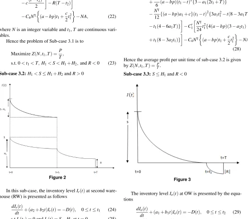
Sub-case 3.2:H1<S≤H1+H2andR>0
Figure 2
In this sub-case, the inventory levelIr(t)at second ware-house (RW) is presented as follows
dIr(t)
dt + (a2+b2t)Ir(t) =−D(t), 0≤t≤t1 (24) s.t.Ir(t1) =0 andIr(t) =S−H1att=0 (25)
The inventory levelIo(t)at first storehouse (OW) in the inter-val[0,T]is presented as follows
dIo(t)
dt + (a1+b1t)Io(t) =0, 0≤t<t1 (26) dIo(t)
dt + (a1+b1t)Io(t) =−D(t), t1≤t≤T (27) s.t.Io(t) =H1att=0 andIo(t) =Ratt=T.
The Total profit (P) for this sub-case is as follows
P=pNγ
(a−bp)T+c 2T
2
−C3(S−R)−(R1+R2)
−C1
H1
t1−a1t 2 1 2
+R(T−t1)
+N γ
6 (a−bp)(t1−t) 2{
3−a1(2t1+T)}
−N
γ
12{(a−bp)a1+c}(t1−t) 2{3a
1t12−t(8−3a1T)
−t1(4−6a1T)}
−C10
Nγ 24t
2
1{4(a−bp)(3−a2t1)
+t1(8−3a2t1)}
−C4Nγ
(a−bp)t1+ c 2t
2 1
−NA
(28)
Hence the average profit per unit time of sub-case 3.2 is given byZ(N,t1,T) =PT.
Sub-case 3.3:S≤H1andR<0
Figure 3
The inventory levelIo(t)at OW is presented by the equa-tions
dIo(t)
dt + (a1+b1t)Io(t) =−D(t), 0≤t≤t2 (29) dIo(t)
dt =−
D(t)
1+δ(T−t), t2<t≤T (30) s.t.Io(t2) =0, Io(0) =SandIo(T) =−R. (31)
Hence the net profit is given by
P=p
Nγ
(a−bp)t2+ c 2t
2 2
+|R|
−C3(S+|R|)
−R1−C1
Nγ 24t
2
2{4(a−bp)(3−a1t2) +t2(8−3a1t2)}
+C2
Nγ δ
a−bp+c
T+1 δ
1
dlog|1+δ(T−t2)|{1+δ(T−t2)} −(T−t2)
−c(t−t2) 2
2
−R(T−t2)
Hence the average profit per unit time of sub-case 3.3 is given byZ(N,t1,T) =TP.
Sub-case 3.4:S≤H1andR>0
The inventory levelIo(t)at first storehouse (OW) is ex-pressed by the following equations
dIo(t)
dt + (a1+b1t)Io(t) =−D(t),0≤t≤T (33) s.t.Io(0) =SandIo(T) =R. (34)
Here the total profit is given by
P=pNγ
(a−bp)T+c 2T
2
−C3(S−R)−R1
−C1
ST
2 (2−a1T)− Nγ
6 t
2(a−bp)(3−2a1T)
−N
γ
24t
3{(a−bp)a
1+c}(4−3a1T)
−NA
(35)
The average profit per unit time is given byZ(N,t1,T) =PT.
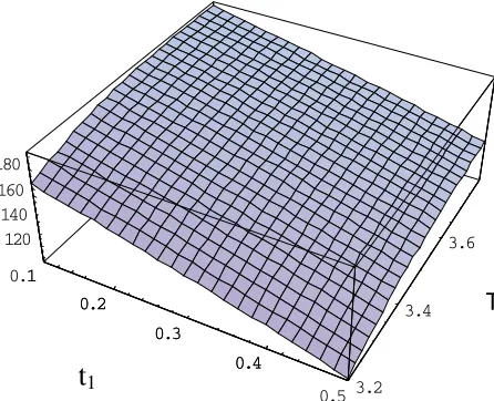
4. Numerical illustration
C1=Re. 1.0/unit/unit time,C2=Rs. 12/unit/unit time, C10 = Rs. 1.5/unit/unit time, R1= Rs. 150/order, R2= Rs.50/order,a1=0.1,a2=0.08,b1=.01,b2=.02,C3= Rs. 25/unit,C4=Rs. 0.5/unit,H1=100;H2=200,a=150, b=3.5,c=5,γ=0.3,A=Rs. 50/advertisement,δ =2.5. We used Mathematica 5.2 to solve this example for deter-mining the optimal values ofN,t1,t2T,S, andRalong with the average profitZ of the system. We obtained the follow-ing results:t1=1.90618,t2=3.19156,N=5,T =3.65979, R=13.7025,S=147.97,Z=202.007
0.1 0.2
0.3
0.4
0.5 3.2 3.4
3.6 120
140 160 180
0.1 0.2
0.3
0.4
t
1T
Figure 4.Represents the Average profit vs.t1andT The profit function Z(N,t1,T)obtained from equation (23) is highly nonlinear so it is very tedious to solve, thus the
concavity of the function is presented numerically. Figure4 represents that the profit function is concave for the above mentioned example.
5. Conclusions
This paper introduces an inventory model with two store-houses of limited space capacity under time dependent de-terioration rate. Here demand rate of the product changes according to (1) number of advertisement, (2) selling price and (3) time. In the model shortages occurs of which only some units are backlogged. To make model more realistic the rate of decay is taken linear in both storehouses. Also the optimal net profit is calculated by solving proposed model for different system parameters. Finally a numerical example is taken to maximize the total profit of the system. By taking more assumptions, such as inflation, learning effects, greening effects etc the model can be better fitted to real world scenar-ios. It can also be analysed further by introducing different preservation technologies in storehouses.
References
[1] R.V. Hartely,Operations Research – A Managerial
Em-phasis, Goodyear Publishing Company, California, CA, 1976.
[2] A. Goswami and K.S. Chaudhuri, An economic order
quantity model for items with two levels of storage for a linear trend in demand, Journal of the Operational Research Society, 43(1992), 157–167.
[3] H. Yang, Two-warehouse inventory models for
deteriorat-ing items with shortage under inflation,European Journal of Operational Research, 157(2004), 344–356.
[4] T. Hsieh, C. Dye and L.Y. Ouyang, Determining optimal
lot size for a two warehouse system with deterioration and shortages using net present value,European Journal of Operational Research, 191(2002), 182–192.
[5] S.K. Goyal and A. Gunasekaran, An integrated
production-inventory-marketing model for deteriorating items,Computers & Industrial Engineering, 28(1995), 755–762.
[6] X. Xu, Q. Bai and M. Chen, A comparison of different
dispatching policies in two-warehouse inventory systems for deteriorating items over a finite time horizon,Applied Mathematical Modelling, 41(2017), 359–374.
[7] A.K. Bhunia, A.A. Shaikh, G. Sharma and S. Pareek,
A two storage inventory model for deteriorating items with variable demand and partial backlogging,Journal of Industrial and Production Engineering, 32(4)(2015), 263–272.
[8] A.K. Bhunia and M. Maiti, An inventory model for
de-caying items with selling price, frequency of advertise-ment and linearly time-dependent demand with shortages, IAPQR Transactions, 22(1997), 41–49.
[9] P.L. Abad, Optimal lot size for a perishable good under
order-ing and lost sale,Computers & Industrial Engineering, 38(2000), 457–468.
[10] W. Luo, An integrated inventory system for perishable
goods with backordering,Computers & Industrial Engi-neering, 34(1998), 685–693.
[11] B. Mondal, A.K. Bhunia and M. Maiti, A model of two
storage inventory system under stock dependent selling rate incorporating marketing decisions and transportation cost with optimum release rule,Tamsui Oxford Journal of Mathematical Sciences, 23(2007), 243–267.
[12] S.L. Chung and H.M. Wee, Pricing discount for a supply
chain coordination policy with price dependent demand, Journal of the Chinese Institute of Industrial Engineers, 23(3)(2006), 222–232.
[13] B. Sarkar and S. Sarkar, Variable deterioration and
de-mand — An inventory model, Economic Modelling, 31(2013), 548–556.
[14] J. Wu, K. Skouri, J.T. Teng and Y. Hu, Two inventory
systems with trapezoidal-type demand rate and time-dependent deterioration and backlogging,Expert Systems with Applications, 46(2016), 367–379.
? ? ? ? ? ? ? ? ?
ISSN(P):2319-3786
Malaya Journal of Matematik
ISSN(O):2321-5666