Paper 04-2019-2

(10.24874/jsscm.2019.13.02.04)

NUMERICAL STUDY ON HEAT TRANSFER IN MULTILAYERED

STRUCTURES OF MAIN GEOMETRIC FORMS MADE OF

DIFFERENT MATERIALS

Roman M. Tatsiy 1_{, Oleg Yu. Pazen} 2_{, Sergiy Ya. Vovk} 3_{, Lubomyr Ya. Ropyak}4_{, Tetiana} O. Pryhorovska5*

1 _{Lviv State University of Life Safety, 35 Kleparivska Street, Lviv, Ukraine}

e-mail: [email protected]

2 _{Lviv State University of Life Safety, 35 Kleparivska Street, Lviv, Ukraine}

e-mail: [email protected]

3 _{Lviv State University of Life Safety, 35 Kleparivska Street, Lviv, Ukraine}

e-mail: [email protected]

4 _{Frankivsk National Technical University of Oil and Gas, 15 Karpatska Street,}

Ivano-Frankivsk, Ukraine e-mail: [email protected]

5 _{Frankivsk National Technical University of Oil and Gas, 15 Karpatska Street,}

Ivano-Frankivsk, Ukraine

e-mail: [email protected]

*corresponding author

Abstract

The article proposed a general research scheme of heat transfer process in multilayer constructions for three basic geometric forms in order to simulate fire distribution. The scheme is based on linear differential equations, the Fourier method and the modified method of Eigen functions. The work considers five different layers’ design and does not take into account internal heat sources. In this regard, a one-parameter family of boundary problems were solved. The authors simulated heat transfer for the Cartesian, cylindrical and spherical coordinates. Structures comprised several materials each having thermal properties varying with temperature.

Keywords: boundary problem, quasi-derivative, Cauchy matrix, Fourier method, eigen function method

1. Introduction

nuclear reactors, etc (Gay 2015, Kumar 2017). There are numerous papers based on two-dimensional thin-layer models and contain analytical and numerical estimates of thermoelastic equilibrium of bodies with layer coatings under the influence of distributed and local thermal and mechanical loading (Yasniy 2017; Yasniy 2013; Shevchuk 2013; Shevchuk 2017). Temperature stresses in bodies with surface inhomogeneities were investigated in papers by Beck (1984), Bulavin (1965), Giere (1965), Hagn (2012). Temperature effect on properties and destruction for energy equipment materials is studied by Kolesov (1992), and Malanchuk (2017).

The subject of the proposed herein article is the heat transfer and diffusion in multilayer structures. This way, a proper understanding of the internal thermal processes in the laminate structures is of paramount importance for preventing their thermal destruction, for controlling directional heat transfer through them, for analysing of thermal stresses and deformation, etc.

Therefore, it is important to have efficient procedures for heat flow and temperature distribution calculating inside multiple layers. An analytical method or numerical simulations are the most spread approaches to get the mentioned above procedures.

Practically, precise analytical solutions (if they are available) may be very mathematically complicated, and this way numerical methods like FDM (Özişik 2017), FEM (Gosz 2017), or BEM (Aliabadi 2002) become increasingly popular because of modern numerical computation and continuous improvement of computer technologies.

However, the analytical methods have some advantages compared to numerical ones:

1) They offer more reliable results and are numerically more efficient;

2) Precise analytical solutions give a deeper physical insight of the studied process than discrete numerical solutions, and show how the thermal behaviour of a multi-layer structure depends on parameters of layers;

3) Precise analytical solutions can be used within verification and comparison of various numerical methods.

These methods are well described in the classic books (Hahn 2012, Lykov 1967) and have been used by many researchers for stationary and non-stationary temperature fields in multi-layer non-uniform structures. They are the orthogonal and quasi-orthogonal expansion technique (Tittle 1965, Bulavin 1965), Green’s function approach (Siegel 1999, Haji-Sheikh 2002), Laplace transform method (Giere 1965, Lu 2013), Fourier transform method (Kayhani 2012), a finite integral transform (Singh 2011), a method of separation of variables and eigen function expansion (Norouzi 2016), for instance.

The solution of heat transfer problem in multilayer structures was obtained for the Cartesian (Tittle 1965, Salt 1963, Mikhailov 2017, Beck 1984, Siegel 1999, de Monte 2002], cylindrical (Kayhani 2012, Norouzi 2016) and spherical coordinate system (Bulavin 1965, Salt 1963). From the viewpoint of partial differential equations, majority of the approaches are based on the variable separation or integral transformations. Their core is determination of eigenvalues of the corresponding boundary eigenvalue problem. However, this problem is not of traditional type because of discontinuous coefficients due to piecewise-homogeneous bodies.

38

The obtained results can be used, for example, in heat transfer study for a multilayer plate and hollow cylinder under conditions of perfect thermal contact between layers.

This idea has already been implemented in the works of Tatsiy (2011) and Semerak (2015). This way, there was the problem of this scheme unification for multilayer structures of any canonical form.

There are many papers devoted to analytical methods of non-stationary temperature field calculation in layered non-uniform structures. In particular, the methods of the Laplace, Fourier and Green functions have been being applied up to now to the multilayer structures (Semerak 2015, Arsenin 1974). Tikhonov (1997) proposed and substantiated a scheme of a mixed problem solution for heat equation with piecewise continuous coefficients depending on a finite interval spatial coordinate. The scheme was based on the reduction method, quasi-derivative concept, and modern theory of linear differential equation systems, Fourier method and modified method of eigen functions.

2. Statement of the problem and its mathematical formulation

A multilayer construction (in Cartesian, cylindrical or spherical coordinate systems) is

considered. Its area is limited by surfaces rr₀. and rr_n , and is divided into n layers.

Each layer is made of isotropic material and has its coefficient of thermal conductivity ,

specific heat capacity с and density



. Temperature initial distribution function 

 

r was

specified depending on the coordinate r and time τ. There is a convective heat exchange with the environment on the outer surfaces, that is, the third kind boundary conditions are met.

The general form of the thermal conductivity differential equations y in Cartesian, cylindrical, and spherical coordinate systems (equations (1), (2) and (3) respectively) are [1, 2]:

     

t r,

   

t r,

с r r r

r r

 

 



    

  

  _  _ (1)

     

t r, 1

   

t r,

с r r r r

r r r

 

 



 _    

 

  _  _ (2)

     

2

   

2

, 1 ,

t r t r

с r r r r

r r

r

 

 



 _    

 

  _  _ (3)

The only difference of these equations is the rlmultiplier if l=0, l=1 and l=2. So, the

equation (1) - (3) are combined into a one-parameter family of differential equations:

     

, 1

   

,

, 0,1, 2

l l

t r t r

c r r r r l

r r

r

 

 



 _     _

 

  _  _ (4)

n particular, particular, if l = 0 is a multilayered flat construction; if l = 1 is multilayer hollow cylinder; if l = 2 is a multilayer hollow ball.

















0 0 0 0

( , ) , ( ) ,

( , )_{n n n}, _n( ) ,

t

r t r

r t

r t r

r               _{ }    _       (5)

and initial condition:

 

, 0

 

.

t r  r (6)

Where  ₀

 

and  _n

 

- the ambient temperature outside of the near-surface heat layers,

and ₀ and _n - heat transfer coefficients on the rr₀ and rr_n.surfaces.

The follow notations will be used: _i - the characteristic function of the semi-open interval



r ri, i1



, that is

1

1

1, [ , )

0, [ , )

i i i

i i r r r

r r r

       _ 

 

1

0 , n i i i r    





1

0

( ) ( ) ,

n

i i i i

c r  r c   



 



  1

0 ( ) , n i i i r     





 _i, ,c_i _i  0 R,  i 0,n1,

 

[1] , df l r

r t



 t r



– quasi derivative [8],

 

[1] , l t r q r 

 - heat flow density.

The problem (4) - (6) solution is considered as the sum of two functions (the reduction method), according to Ropyak L. Ya., Shatskyi I. P., Makoviichuk M. V.:

 

,

   

, ,

t r



u r



v r



(7)

Any function u r

 

,



or v r

 

, can be chosen in a special way, so another one is determined

unambiguously.

3. u r

 

, function selection and the mixed task

The function u r

 

,



is defined as a solution (quasistationary) of the boundary value

problem:





1

0

l l r u r 



  (8)

















0 0 0 0

( , ) , ( ) ,

( , )_{n n n}, _n( ) ,

u

r u r

r u

r u r

r               _{ }    _       (9)

Where τ – parameter.

The boundary conditions (9) can be rewritten as:

















[1]

0 0 0 0 0 0 0

[1]

, , ( ),

, , ( ),

l l

l l

n n n n n n n

r u r u r r

r u r u r r

     

     

  



 _{ }

40

Where

 

[1] ,

df l u r



r u





..

Based on the (7) projection, the equation (4) is rewritten as:

 

,

 

, 1 l

 

, 1 l

 

,

l l

u r v r u r v r

c c r r

r r r r

r r

   

   

 

       

     

   _  _  _  _ (11)

Assuming u r

 

,



is the solution of the problems (8), (10), and considering

 

,

1

0

l l

u r r

r r

r





 

 _

 

 _  _ in the (11), we receive a non-uniform differential equation for the

functionv r

 

, :

 

, 1 l

 

,

 

,

l

v r v r u r

с r с

r r

r

  

  

 

 _    _ 

 

  _  _  (12)

The function с u r

 

,

  

 at the right-hand side of the equation (12) is considered defined,

that is the function u r

 

,



is defined, too. The function u r

 

,



is considered (8), (10) problem

solution. As far as the function u r

 

,



meets the boundary conditions (10), the projection (7)

defines the boundary conditions for the function v r

 

, .

















[1]

0 0 0 0

[1]

, , 0,

, , 0,

l

l

n n n n r v r v r r v r v r

  

  

  



 _{ }

 (13)

and the initial condition is the following:

 

, 0

 

   

, 0 .

v r  f r 



r u r (14)

Consequently, the function v r

 

, is the solution of the mixed problem (12) - (14), if only

 

,

u r



function is defined as the (8), (10) problem solution.

4. The (8), (10) boundary problem solving

The quasi-derivative concept [4, 8] is used for the problem (8), (10) solving.

The vector



[1]



,

T

U u u and the matrix

1 0

.

0 0

l A r



 

 

 _ _

 

are introduced. This way, the

quaside-differential equation (8) is reduced to an equivalent system of 1-st order differential equations:

U AUR (15)

 

0

 

n

 

,

P U r



 

Q U r

 



(16)

Where

P

and Q  square matrixes:

0 0 1 _, 0 0 _,

1

0 0

l

l n n r

P Q

r





    

   

 

  (17)

And the vector



 



is



₀l _{0 0}

 

, l

 



T.

n n n

r   r  

The function

U r

 

,

which is absolutely continuous on the interval



r r₀, _n



, and fits the this

system almost everywhere (the only exception is, perhaps, the function rupture points

( ), ( ), ( )

c r  r  r ).

The system (15) is:

1 0 ,

0 0

l

i _i

i i i r

U A U A 

 

 

  _{  }

 

 

(18)

for each interval.

The Cauchy matrix [4-7] B_{i l,}( , )r s of the system (18) is the follows:

 

, ,

1 ,

( , ) , 0,1, 2,

0 1

i l i l

K r s B r s _ _ l

  (19)

where

 

,

1 ,

r

i l l

i s dz K r s

z





_

(20)

For arbitrary ki, it was designated

1, 1 2, 1 2 , 1

( , ) ( , ) ( , ) ... ( , ),

df

l n m n l n n n l n n m l m m

B r r B r r B r r  B r  r nm (21)

Assuming B r r_l( ,_{m m})E, where

E



is a 2 2. matrix.

The structure (19) of the matrices Bi l_,

 

r s, makes possible to establish the matrix structure

(21), in particular:

 

1 ,

1 ,

( , ) ,

0 1

n i l i m l n m

K r s

B r r n m





 

 

_{ } 

 

 



₍₂₂₎

The work [4, 6] stated that the vector function U ri( ) is the solution of problem (15) for each

interval.

0 0

( ) ( , ) ( , )

i _{i i i i}

U r B r r B r r  P



(23)

42

1 0 ( l( , ))n 0

P  P QB r r   (24)

and the matrices are defined in (17) and the matrices

P

and Qare defined in (17).

It should be noted that the decision function u r_i( ) is the first coordinate of the

vector-function U ri( ) (problem (8), (10)); and its quasi-derivative is the second coordinate u[1]_i ( )r . The

solution (23) of the problem (8), (10) exists and is unique when the condition



0



det P QB r r l( , )n 0is fulfilled.

The expression (23) makes possible to define a solution over the entire interval



x x₀, n



using

characteristic functions _i as:

 

1

 

0

, , .

n

i i i

u r u r 









(25)

5. Fourier method and task for eigenvalues

We search non-trivial partial solutions of the homogeneous differential equation:

 

, 1 l

 

,

l

v r v r

c r

r r

r

 

 



   

  

  _  _ (26)

which fulfils the boundary conditions (13), in the form [9]

( , ) ( )

v r eR r (27)

where  – parameter, R r

 

– unknown function.

The follow quasi-differential equation was obtained by substituting the right-hand side of (27) in (26):



rl



R 





 

c r Rl 0 (28) with boundary conditions:

[1]

0 0 0 0

[1]

( ) ( ) 0,

( ) ( ) 0.

l l

n n n n r R r R r r R r R r

 

  

 

 

 (29)

The problem (28), (29) is a classical eigenvalue problem for  parameter (eigenvalues)

definition, which corresponds to nontrivial solutions (own functions) Rk



r,k



. Properties of

eigenvalues _k and their own functions Rk



r,



k



are exhaustively studied and described in

6. Structural construction of own functions

We introduce the following notation:  1

df l

R rR – quasi-derivative, vector



,  1



T

R R R and

matrix 1 0 0 l l A r r c



 

     _ _    .

Then the quasi-differential equation (28) is reduced to the system of equivalent first order differential equations:

R

 

AR

(30)

The corresponding system on the interval



r r_i,_i1



is:

, 0, 1,

i i i

R A R i n (31)

Where Ai - the matrix

1 0 0 l i _i l i i r A r c         _ _    .

As it was mentioned above, absolutely continuous vector-function

R r

 

,



is the solution of

the system (30), which corresponds to the conditions of the ideal thermal contact between the layers.

The Cauchy matrix

B

i l,



r s

, ,





of the system (31) is:

       

          

       

          

,

1 0 0 1 0 0 0 0

2

1 1 1 1 1 0 0 1

( , , ) sin ( ) cos ( )

, 0 sin ( ) cos ( )

, , , , , , , , 2 2 , , , , , , , , 2 2 i l i i i i

i i i i

i i i i i i i i i

i

i i i i i i i i i i

B r s

r s r s

l

r s r s

s J s Y r J r Y s J s Y r J r Y s

rs J r Y s J s Y r r J r Y s J s Y r                                         _{ }                                       , 1

cos sin sin

, 2

sin cos cos sin

i i i i

i i i

i i i i i i i i i i

i i

l

s r s r s r s

r rs

l

c rs r s s r r s r r s r s

s                                                 _   _   _{ }     _ _   _                      _{ }  _{ }    (32)

Where i i

i i c    

 , J₀ and N₀–the Bessel and Neumann functions of zero order respectively.

44

1 ₁ 2 _{1 2 1}

( , , ) ( , , ) ( , , ) ... ( , , ) ,

df

k k i

k i k k k k i i

B r r  B  r r_  B  r_ r_   B r_ r  ki (33)

Let's also mark





1



 



,

0 0

0

, , , , , , ,

n df

l i l _i l _{i i}

i

B r r  B r r  B r r  









  (34)





11

 

_{ }

12

 

_{ }

0

21 22

, , .

df l n

b b

B r r

b b

 



 

 

 

  (35)

The non-trivial solution

R r

 

,



of the system (30) is found as

 

,

l



, ,

0



,

R r





B r r





C

(36)

where C



C₁, C₂



Ta non-zero vector.

Applying to both parts of equality (36) boundary conditions in the form (16) for



 





0,

it was obtained:



0,





n,



l



0, ,0



l



n, ,0



0,

P R r   Q R r  _P B r r   Q B r r  _ C

or, assuming

B r r

_l



₀

, ,

₀

 



E

,

where

E

– unit matrix:



, ,0



0

l n

P Q B r r  C

    

  (37)

The necessary and sufficient conditions for a nonzero vector Cin (37) are:



0



det_P Q B r r  _{l n}, , _0. (38)

We can define the form of the left (characteristic) equation (38), considering the formulas (17) and (35)





0 0 11

 

_{ }

12

 

_{ }

0

21 22

0 0

1

det , , det 0

1

0 0

l

l _{n l}

n n

b b

r P Q B r r

r b b















      

        

  _{     }

 

So we got the result, which we will formulate in the form of

Statement 1. The characteristic equation of the problem for eigenvalues (28), (29) has the form

 

 





 

 

0 0 12 22 11 21 0

l l l

n n n n

r



r



b



b



r



b



b



 (39)

As it is known [9], the roots of the characteristic equation _k (39) are positive and different.

They are the eigenvalues of the problem (28), (29).

To find a nonzero vector C



C₁, C₂



Twe substitute _k in (37) instead of . Then we

11 12 1 0 0

21 22 2

0 1

11 21 12 22 2

0 0 ( ) ( ) 0

1

,

1 ( ) ( ) 0

0 0

1 0

( ( ) ( )) ( ( ) ( )) 0

l

k k

l

n n k k

l l

n n k k n n k k

b b C

r

r b b C

C

r b b r b b C

                                                      _{  } _{  }   _{   }  

which is equivalent to the system of equations

0 0 1 2

11 21 1 12 22 2

0,

( ( ) ( )) ( ( ) ( )) 0.

l

l l

n n k k n n k k

r C C

r b b C r b b C















          

 (40)

As far as the system determinant is equal to zero, then system (40) has non-zero solutions

1 0, 2 0

C  C   . Assuming, for instance C₂ 1,

0 0 1

, 1 .

T l C r



    

  (41)

By denoting a non-trivial eigenvector corresponding to its Eigen value k_{, we obtain}

Statement 2. Eigenvector of the system of differential equations (30) with boundary

conditions (16) for



 





0,

has the following structure







 

0



0 0

1

, , , , , , 0, 1

1

l ki _{k il i k l i k} r

R r B r r  B r r   i n

      _{ }       (42)

Consequence. Eigen functions Rk



r,



k



, as the first coordinates of eigenvectors



,



k _k

R

r



, can be written as:







0



0 0

1

, (1, 0) , , , 1,

1

l

k k l k r

R r B r r   k

      _{ }       (43)

In particular, since









1

0

, , ,

n

k k ki k i i

R r  R r   







it follows from (43) that







 

0



0 0

1

, (1;0) , , , , , 0, 1

1

l ki k il i k l i k r

R r B r r  B r r   i n

       _{ }       (44)

7. Development in the Fourier series by Eigen functions Rk



r,



k



Let’s assume 1 0 ( ) ( ) n i i i

g r g r





46

Is a piecewise-absolutely continuous function, defined at the



r r₀, _n



interval, specified by

the different analytical expressions g r_i( )on each of the interval



r r_i,_i1



. In particular, the

function g r

 

is developed in the Fourier series by its Eigen functions R_k



r,



_k



of the problem

(28), (29) [4]:

1

( ) k k( , k)

k

g r g R r 









(46)

where the Fourier coefficients g_k are calculated by the formulas

1

1 2

0 1

( ) ( , )

|| ( , ) ||

i

i

r n

l

k i i i ki k

i

k k r

g c r g r R r dr

R r   

 







_

  (47)

2

k

R  Eigen function norm square R_k



r,



_k



, which is calculated by the formula

1

1

2 2

0

|| ( , ) || ( , )

i

i

r n

l

k k i i ki k i r

R r c r R r dr

 







_

 (48)

8. Development of a mixed problem (8), (9), (10) solution

The Eigen function method [10] was used to solve the problem (12) - (14). It means the problem (12) - (14) is solved as

 

 





1

, k k , k ,

k

v r T  R r









 (49)

where Tk

 



 unknown functions that we will define later.

As far as u





 is included into the right-hand side of equation (12), we will develop it in the

Fourier series by its Eigen functions (43) of the boundary problems (28) - (29), and the variable

 is a parameter.

Substituting (49) into (12) and after transformations we obtain an infinite set of equations

 

 

 

0, 1, 2, 3,....

k k k k

T  T  u   k (50)

where u_k

 

 – Fourier coefficients of development.

 





1

,

k k k

k

u

u



R r











_

_





(51)

The general solution of the differential equation (50) for each k is:

 

 

_{ }

0

,

k

k s

k k k

T t f e e u s ds

  

   



  

_

 (52)

 





1

( ) ( , 0) _{k k} , _k

k

f r  r u r f R r





  



(53)

Finally we obtain the solution of the mixed problem (12) - (14) as the vector-function

 

 

_{ }

_

_

1

_{ }

1 0 0

, k k , ,

n s

k

k k k i i

k i

V r f e e u s ds R r V r

    

        

 

 

 _   _ 

 







(54)

where the first coordinate v r

 

, is the desired function, and the second one [1]

 

,

v r is its

quasi-derivative.

The solution of the mixed problem (12) - (14) is obtained in the form of a series:

 

 

_{ }

_

_

1 0

, k k s ,

i k k ki k

k

v r f e e u s ds R r

    

     



 

 _   _

 





(55)

on each of the interval.

Taking into account (25) and (55), we obtain the solution (7) of the problem (4) - (6)

 

1

 

 

0

, , , ,

n

i i i

i

t x u x v x 









_  _ (56)

9. Numerical implementation of the method (model example)

As a numerical example, we consider a construction that consists of five different layers. There is a convection heat exchange with the environment on its surfaces. It is necessary to determine the distribution of the non-stationary temperature field of the five-layer structure (for Cartesian, cylindrical and spherical coordinate systems), if, on the one hand, the temperature changes according to the law of the standard fire temperature regime (Buketov A V, Dolgov NA,

Sapronov A A et al.). At the initial time, temperature is constant 0

20 C. The thermophysical

48

Option Layer 1 Layer 2 Layer 3 Layer 4 Layer 5

Thickness, [m] 0.05 0.2 0.03 0.06 0.01

Coefficient of thermal

conductivity [W/m2 _·0_С] 0.76 1.92 0.09 0.7 0.96

Specific heat [J/ kg0_{С] 840 840 840 840 880}

Density 1800 2500 300 1600 2000

Temperature change laws

 

0

 

20,

 

8

345 lg 1 20

60

n



   _  _

 

Coefficients of heat transfer

on surfaces 0 25, n 4

Table 1. Initial data for problem solving

We have obtained non-stationary temperature field problem solution for the five-layer construction for different coordinate systems by the proposed method.

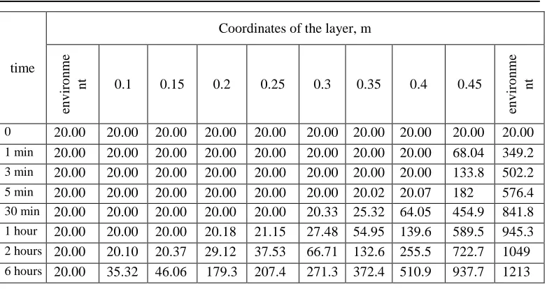
Cartesian coordinate system (five-layer flat wall)

time

Coordinates of the layer, m

en

v

ir

o

n

m

e

n

t _{0.1 0.15 0.2 0.25 0.3 0.35 0.4 0.45}

en

v

ir

o

n

m

e

nt

0 20.00 20.00 20.00 20.00 20.00 20.00 20.00 20.00 20.00 20.00

1 min 20.00 20.00 20.00 20.00 20.00 20.00 20.00 20.00 68.04 349.2

3 min 20.00 20.00 20.00 20.00 20.00 20.00 20.00 20.00 133.8 502.2

5 min 20.00 20.00 20.00 20.00 20.00 20.00 20.02 20.07 182 576.4

30 min 20.00 20.00 20.00 20.00 20.00 20.33 25.32 64.05 454.9 841.8

1 hour 20.00 20.00 20.00 20.18 21.15 27.48 54.95 139.6 589.5 945.3

2 hours 20.00 20.10 20.37 29.12 37.53 66.71 132.6 255.5 722.7 1049

6 hours 20.00 35.32 46.06 179.3 207.4 271.3 372.4 510.9 937.7 1213

Table 2. Distribution of the temperature field of a five-layer flat structure, 0_С

time

Coordinates of the layer, m

0.1 0.15 0.2 0.25 0.3 0.35 0.4 0.45

0 0 0 0 0 0 0 0 0

1 min 0 0 0 0 0 0 0 7029

3 min 0 0 0 0 0 0 0 9211

5 min 0 0 0 0 0 1.7 16.48 9860

30 min 0 0 0 0 41.6 496.5 3057 9673

1 hour 0 0 1.6 90.8 490.5 1854 4978 8896

2 hours 0.2 8.8 37.7 646.9 1700 3498 6039 8159

6 hours 61.1 252 410.8 1754 3161 4605 6024 6898

Table 3. Distribution of the density of the heat flow of a five-layer flat construction, W/m2

50

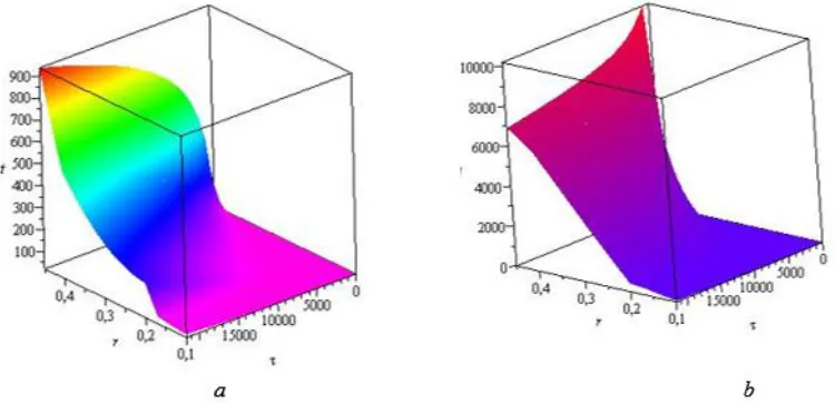
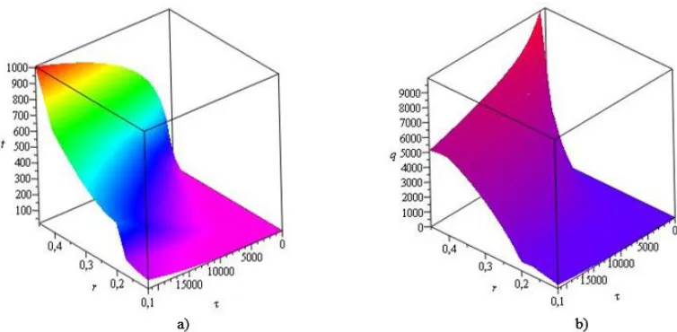
Fig. 2. Volume distribution: a - temperature field; b - heat flow density

time

Coordinates of the layer, m

en

v

ir

o

n

m

en

t _{0.1 0.15 0.2 0.25 0.3 0.35 0.4 0.45}

en

v

ir

o

n

m

en

t

0 20.00 20.00 20.00 20.00 20.00 20.00 20.00 20.00 20.00 20.00

1 min 20.00 20.00 20.00 20.00 20.00 20.00 20.00 20.00 68.19 349.2

3 min 20.00 20.00 20.00 20.00 20.00 20.00 20.00 20.00 134.6 502.2

5 min 20.00 20.00 20.00 20.00 20.00 20.00 20.00 20.08 183.4 576.4

30 min 20.00 20.00 20.00 20.00 20.00 20.39 26.15 67.96 462.3 841.8

1 hour 20.00 20.00 20.00 20.48 21.64 29.5 61.03 151.9 601.6 945.3

2 hours 20.00 20.13 20.58 33.48 44.44 80.04 154.4 283.8 741.4 1049 6 hours 20.00 49.68 67.09 243.9 277.2 348.3 453.1 587.6 973.7 1213

time

Coordinates of the layer, m

0.1 0.15 0.2 0.25 0.3 0.35 0.4 0.45

0 0 0 0 0 0 0 0 0

1 min 0 0 0 0 0 0 0 7023

3 min 0 0 0 0 0 0 0 9192

5 min 0 0 0 0 0 0 19.65 9824

30 min 0 0 0 0 50.3 560.1 3222 9487

1 hour 0 0 2.51 119 590.4 2069 5193 8593

2 hours 1.5 14.5 51.76 829.8 2001 3820 6170 7692

6 hours 118.8 377.3 504.9 2040 3401 4623 5678 5996

Table 5. Distribution of the temperature field of a five-layer cylindrical structure, 0_С

Spherical coordinate system (five-layer hollow sphere)

52

time

Coordinates of the layer, m environme

nt 0.1 0.15 0.2 0.25 0.3 0.35 0.4 0.45

environme nt

0 20.00 20.0

0 20.0 0 20.0 0 20.0 0 20.0 0 20.0 0 20.0 0 20.0 0 20.00 1 min

20.00 20.0

0 20.0 0 20.0 0 20.0 0 20.0 0 20.0 0 20.0 0 68.3 9 349.2 3 min

20.00 20.0

0 20.0 0 20.0 0 20.0 0 20.0 0 20.0 0 20.0 0 135. 4 502.2 5 min

20.00 20.0

0 20.0 0 20.0 0 20.0 0 20.0 0 20.0 0 20.0 6 184. 8 576.4 30 min

20.00 20.0

0 20.0 0 20.0 0 20.0 0 20.5 1 27.0 9 72.0 9 469. 7 841.8 1 hour

20.00 20.0

0 20.1 8 20.7 8 22.1 7 31.8 6 67.8 3 164. 8 613. 7 945.3 2 hour s

20.00 20.4

3 21.1 5 39.2 5 53.3 6

96 178.

8 313. 7 760. 1 1049 6 hour s

20.00 73.7

7

99.9 2

320 358.

1 433. 8 538. 5 665. 6 100 8 1213

Table 6. Distribution of the temperature field of a five-layer hollow sphere, 0_С

time

Coordinates of the layer, m

0.1 0.15 0.2 0.25 0.3 0.35 0.4 0.45

0 0 0 0 0 0 0 0 0

1 min 0 0 0 0 0 0 0 7022

3 min 0 0 0 0 0 0 0 9172

5 min 0 0 0 0 0 0 18.61 9790

30 min 0 0 0 0 61.35 628.5 3389 9301

1 hour 0 1.2 3.01 154.7 704.3 2294 5399 8290

2 hours 1.4 22.7 68.73 1041 2316 4124 6259 7226

6 hours 214.8 526.2 584.4 2256 3509 4491 5229 5129

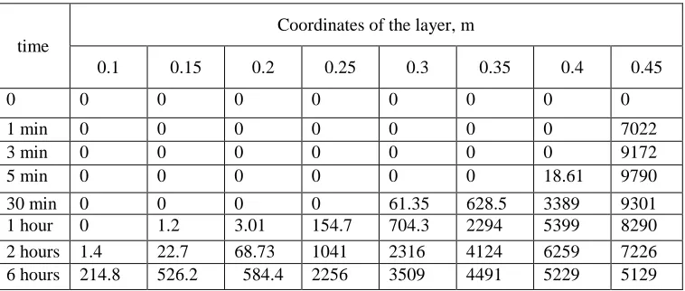
Table 7. Distribution of heat density of a five-layer hollow ball, W/m2

10. Conclusions

relations. The presented examples use only the standard temperature mode of fire to show the proposed method application. The obtained analytical solution is modelled as a pseudocode and implemented on a specific numerical example.

Acknowledgements The authors are grateful to all the teams of Ivano-Frankivsk National University of Oil and Gas (Ukraine) and Lviv State University of Life Safety for sharing their pearls of wisdom of this research, and thanks the reviewers for their insights.

References

Aliabadi M H (2002). The Boundary Element Method, Applications in Solids and Structures,

John Wiley & Sons, 598.

ArseninVYa (1974).Methods of Mathematical Physicsand Special Functions, Nauka, Moscow.

Beck J V (1984). Green’s Function Solution for Transient Heat Conduction Problems, Int. J. Heat

Mass Transfer, Vol. 27, Issue 8. 1235–1244.

Buketov A V, Dolgov N A, Sapronov A A et al (2017). Mechanical Characteristics of Epoxy

Nanocomposite Coatings with Ultradisperse Diamond Particles. Strength Mater, 49,

464-471.

Bulavin P E, Kascheev V M (1965). Solution of the non-homogeneous heat conduction equation

for multilayered bodies, Int. Chem. Eng, Vol. 1, Issue 5, 112–115.

Dolgov M A, Zubrets’ka N A, Buketov A V et al. (2012). Use of the method of mathematical experiment planning for evaluating adhesive strength of protective coatings modified by

energy fields, Strength Mater, 44(1), 81-86.

EN 1991-1-2 (2002). (English): Eurocode 1: Actions on structures – Part 1-2: General actions – Actions on structures exposed to fire Authority: The European Union Per Regulation 305/2011, Directive 98/34/EC, Directive 2004/18/EC.

Gay, D (2015). Composite Materials: Design and Application, 3rd Edition. New York: CRC

Press, 635

Giere A C (1965). Transient Heat Flow in a Composite Slab — Constant Flux, Zero Flux

Boundary Conditions, Appl. Sci. Research, Section A, Vol. 14, Issue 1, 191–198.

Gosz M R (2017). Finite Element Method: Applications in Solids, Structures, and Heat Transfer,

New York: CRC Press, 400.

Hahn D W, Özişik M N (2012). Heat Conduction, New York: John Wiley & Sons, 744.

Haji-Sheikh A, Beck J V (2002). Temperature solution in multidimensional multi-layer bodies,

Int. J. Heat Mass Transfer, Vol. 45, Issue 9, 1865–1877.

Jain P.K., Singh S., Rizwan-uddin (2010). An exact analytical solution for twodimensional,

unsteady, multilayer heat conduction in spherical coordinates, Int. J. Heat Mass Transfer,

Vol. 53, Issue 9-10, 2133–2142.

Kayhani M H, Norouzi M, Amiri Delouei A (2012). A general analytical solution for heat

conduction in cylindrical multilayer composite laminates, Int. J. Therm. Sci, Vol. 52, Issue

1, 73–82.

Kolesov V S, Vlasov N M, Tisovskii L O, Shatskii I P (1992). The stress-deformation state of an

elastic half-space with a spheroidal thermal inclusion, International Applied Mechanics,

28(7), 426-434.

Kolodziejczyk W, Kul’chyts’kyi-Zhyhailo R (2007). Pressure of the lateral surface of a cylinder

on a periodically layered half space. Mater Sci, 43, 351-360.

Kolyano Yu M, Protsyuk B V, Sinyuta V M, Shebanov S M, Sharov S M (1992). Non-stationary

temperature field in a multilayer orthotropic cylinder, Engineering Physics Journal, Vol. 62,

54

Kul’chyts’kyi-Zhyhailo, R.D. (2012). Elastic half space with laminated coating of periodic

structure under the action of Hertz's pressure. Mater Sci, 47: 527-534.

Kumar M (2017). Applications of Composite Materials, Arcler Education Incorporated, 273.

Li M, Lai A C K (2013). Analytical solution to heat conduction in finite hollow composite

cylinders with a general boundary condition, Int. J. Heat and Mass Transfer, Vol. 60,

549-556.

Lu X, Tervola P, Viljanen M (2005). A new analytical method to solve heat equation for

multi-dimensional composite slab, J. Phys. A: Math. Gen, Vol. 38, Issue 13, 2873–2890.

Lu X, Tervola P, Viljanen M (2006). Transient analytical solution to heat conduction in composite

circular cylinder, Int. J. Heat Mass Transfer, Vol. 49, Issue 1-2, 341–348.

Lykov A V (1967). Heat Conduction Theory, Moscow: Vysshaya Shkola.

Malanchuk N I, Slobodyan B S, Martynyak R M (2017). Friction Sliding of Elastic Bodies in the

Presence of Subsurface Inclusions, Mater Sci, 52, 819-826.

Mikhailov M D, Özişik M N (2017). Transient conduction in a three-dimensional composite slab,

Int. J. Heat Mass Transfer, Vol. 29, Issue 2, 340–342.

Monte F de (2002). An analytic approach to the unsteady heat conduction processes in

one-dimensional composite media, Int. J. Heat Mass Transfer, Vol. 45, Issue 6, 1333–1343.

Monte F de (2003). Unsteady heat conduction in two-dimensional two slab-shaped regions. Exact

closed-form solution and results, Int. J. Heat Mass Transfer, Vol. 46, Issue 8, 1455–1469.

Norouzi M, Rahmani H, Birjandi A K, Joneidi A A (2016). A general exact analytical solution

for anisotropic non-axisymmetric heat conduction in composite cylindrical shells, Int. J. Heat

Mass Transfer, Vol. 93, 41-56.

Özişik M N, Orlande H R B, Colaço M J, Cotta R M (2017). Finite Difference Methods in Heat Transfer, Second Edition. New York: CRC Press, 580.

Ropyak L Ya, Shatskyi I P, Makoviichuk M V (2017).Influence of the oxide-layer thickness on

the ceramic-aluminium coating resistance to indentation. Metallofizika i Noveishie

Tekhnologii. 2017. 39(4): 517-524.

Salt H (1983). Transient conduction in a two-dimensional composite slab-I. Theoretical

development of temperature modes, Int. J. Heat Mass Transfer, Vol. 26, Issue 11, 1611–

1616.

Semerak M M, Tatsii R M, Pazen O Y (2015). Multilayer thermal insulation capacity construction

with regard to damage arbitrary layer, Vestnik Kokshetauskogo tekhnicheskogo instituta,

Issue 4, 8-17.

Shats’kyi І P, Ropyak L Y, Makoviichuk M V (2016). Strength optimization of a two-layer coating for

the particular local loading conditions, Strength of Materials, 48(5), 726-730.

Shevchuk V A (2017). Thermoelasticity problem for a multilayer coating/half-space assembly

with undercoat crack subjected to convective thermal loading. Journal of Thermal Stresses,

40(10), 1215-1230.

Shevchuk V A (2013). Analytical solution of nonstationary heat conduction problem for a

half-space with a multilayer coating, J Eng Phys Thermophy, 86(1), 450-459.

Siegel R (1999). Transient thermal analysis of parallel translucent layers by using Green’s

functions, J. Thermophys. Heat Transfer (AIAA), Vol. 13, Issue 1, 10–17.

Singh S, Jain P K, Rizwan-uddin (2011). Finite integral transform method to solve asymmetric

heat conduction in a multilayer annulus with time-dependent boundary conditions, Nucl.

Eng. Des, Vol. 241, Issue 1, 144–154.

Tatsii R M, Stasiuk M F, Mazurenko V.V, Vlasii O O (2011). Generalized equation

kvazidyferentsialni, Prepr./AN Ukraini IPPMM; No 2-94, 1-4.

Tatsiy R. M., Pazen O. Y. (2015). Direct method for calculating a non-stationary temperature

field under fire conditions, Pozhezhna bezpeka: Zb. nauk. Pr, Lviv: LDU BZHD, Issue 26,

Tatsiy R M, Pazen O Y (2016) General boundary-value problems for the heat conduction equation

with piecewise-continuous coefficients, Journal of Engineering Physics and Thermophysics,

Vol. 89, Issue 2, 357-368.

Tatsiy R M, Stasiuk M F, Vlasii O O, Pazen O Yu (2017) The direct method of studying the temperature field in a multilayer pipeline under fire conditions, Information Technologies

and Computer Modeling, Collection of articles of the International scientific and practical

conference, May 15-20, 436-440.

Tikhonov A N, Samarskii A A (1977) Mathematical physics equation, Nauka, Moscow, 735.

Tittle CW (1965). Boundary value problems in composite media: quasiorthogonal functions, J.

Appl. Phys, Vol. 36, Issue 4, 1486–1488.

Tokovyy Y., Ma C.-C. (2015) Analytical solutions to the axisymmetric elasticity and

thermoelasticity problems for an arbitrarily inhomogeneous layer, International Journal of

Engineering Science, 92 (1), 1-17.

Yasniy O, PyndusYu,YasniyV, LapustaY (2017). Residual lifetime assessment of thermal power plant superheater header, Engineering Failure Analysis, 82(10), 390-403.

Yasniy O, Vuherer T, Yasniy V, Sobchak A. (2013). Mechanical behaviour of material of thermal power

plant steam superheater collector after exploitation, Engineering Failure Analysis, 27(1), 262-271

Yasniy V, Maruschak P, Yasniy O. Lapusta Y (2013). On thermally induced multiple cracking of a