ISSN: 2334-2382 (Print), 2334-2390 (Online) Copyright © The Author(s). 2015. All Rights Reserved. Published by American Research Institute for Policy Development DOI: 10.15640/jeds.v3n1a4 URL: http://dx.doi.org/10.15640/jeds.v3n1a4 The Shilnikov Saddle-Node Bifurcation in a Monetary Policy with
Endogenous Time Preference
Giovanni Bella1
Abstract
We improve the analysis made in Chang et al (2011), by exploring the possibilities for the raise of global indeterminacy via a Shilnikov saddle-node bifurcation on an invariant circle. This allows us to better understand the determinants for the emergence of endogenous fluctuations in a monetary policy model, and to explain the existence of irregular patterns. Hence, the economy may start at some point to oscillate around the long run equilibrium, and eventually deviate from its saddle-path stable solution, thus locating the economy in a particular optimal converging path that could not coincide with the one corresponding to the lowest desired interest rate.
Keywords: Monetary policy, global indeterminacy, Shilnikov saddle-node bifurcation
JEL classification: E52, E31, O11, O41, O42, Q56
1. Introduction
A bulk of literature is concerned with the capacity of monetary policy to stabilize the economy by ensuring the uniqueness of equilibrium. In the last two decades, paramount studies have shown that when the monetary authority decides to raise the nominal interest rate less than the increase in inflation (commonly known as a passive interest rate feedback rule), this might destabilize the economy by inducing fluctuations, and thus render the equilibrium indeterminate (see, Benhabib et al, 2001; Dupor, 2001). Most of these analyses simply consider a constant rate of time preference.
1
One exception in found in Chang et al. (2011) who extend the Benhabib et al. (2001) model by exploring the role played by endogenous time preference in destabilizing the economy under monetary policy actions. Specifically, they find that either an active or a passive interest rate feedback rule can generate local indeterminacy of the equilibrium, which is in sharp contrast with the existing literature on the field.
More interestingly, recent literature is exploring the possibilities for the raise of global indeterminacy, where the economy may start at some point to follow completely different equilibrium paths towards the long-run steady state. The main implication for any policy decision is that if global indeterminacy occurs, public intervention becomes not sufficient to drive the economy towards a good long-run equilibrium. The agents' decisions, despite the initial conditions or other economic fundamentals, will locate the economy in a particular optimal converging path that could not coincide with the one corresponding to the lowest desired monetary policy. To date, only very few attempts have been made to analyze the conditions under which these indeterminacy problems arise outside the small neighborhood of the steady state (Mattana et al. 1999). The latter seems an innovative field to work on, even though it is usually related to very complicated nonlinear functions which increase the mathematical difficulties in handling these models.
The paper develops as follows. The second Section introduces the dynamic system associated with Chang et al. (2011). In the third Section, we prove the main proposition relating to the global properties of the equilibrium, and show the parametric onset for the emergence of global indeterminacy and the saddle-node dynamics. A brief conclusion reassesses the main findings of the paper, and a subsequent Appendix provides all the necessary proofs.
2. The Model
Assume that the economy consists of an infinitely lived representative household and a government, as in Chang et al. (2011). Time is continuous. Each household is endowed with one unit of labor (which is supplied inelastically), and derives utility from consumption, c, and real money holdings, m.
To begin with, let the utility function be defined as
0 ( , )
U
u c m e dt (1)Where
0 ( , )
t
u c m ds
(2)is the cumulated subjective discount rate, depending on the instantaneous subjective discount rate, ( )u , at time s. Hence
u (3)
where the dot stands for time derivative.
The government budget constraint is finally given by
( )
a y R aRm c (4)
where a represents the total real wealth, R is the nominal interest rate, is the inflation rate, and measures exogenous lump-sum taxes.
0
max u c m e dt( , )
. .
( )
s t
a y R a Rm c
u
which implies the following Hamiltonian function
( , ) ( )
H u c m y R aRm c u (5) where and are the costate variables.
Assuming an endowment of physical capital, k, production occurs according to the following functional relationship
( )
y f k (6)
which is assumed strictly increasing and concave in k, i.e., fk 0 and fkk 0
Solution to the optimization problem allows too btain the following third-order autonomous system of differential equations
( )
( , )
( ) ( , , )
k
f k u c m
k f k c k
(S)
Linearization of (S ) around the equilibrium, and straightforward computations leads to
( ) fkck
Tr J (8)
( ) (1 ) ( )
( 1)
kk mm c m
f u u u
Det J (9)
( ) (u cc u mm c f kk) (fkck)
B J (10)
Remark 1 Chang et al. (2011) points out that: (i) the equilibrium is determinate under an active interest rate feedback rule
1
; (ii) the equilibrium is determinate if the monetary authority implements an aggressively passive interest-rate feedback rule
1
, while it may be either indeterminate or unstable if the
monetary authority implements a moderately passive interest-rate feedback rule
1 1
.
Specifically, an active interest-rate feedback rule
1
implies that theinflation rate must fall. Hence households increase their money holding, whereas the time preference rate rises as well. As a consequence, the equilibrium solution is locally determinate. Alternatively, if monetary policy is passive
1
, a lower real interestrate is associated with an increase in inflation rate. This drives households to decrease their money holding, so that the time preference rate will fall. Finally, when the monetary authority implements a moderately passive interest-rate feedback rule
( )
(1 ) 1
, the effect of a reduction in the time preference rate will dominate the
fall in the real interest rate, and consequently an indeterminate solution occurs.
3. The Shilnikov Saddle-Node Bifurcation
The bifurcation analysis provides several instruments to this end. To ease the mathematical computation, we can transform system (S) into a more convenient Jordan normal form in cylindrical coordinates (r z, ,):
3 2
1 2 3
2 2 3 2
1 2 3 4
2 2
1 2 3
r a rz a r a rz
z b r b z b z b r z
c z c r c z
(11)
whose three-dimensional dynamics is topologically equivalent to the evolution of the original vector field in S (see, Wiggins, 1991).
In particular, r describes the amplitude of the limit cycle oscillations in the vicinity of the Hopf bifurcation. Noticeably, the first two equations are independent of , which describes a rotation around the r-axis with almost constant angular velocity , for any | |r small. Thus, we can restrain the analysis to a simpler two-dimensional vector field, which is often called a truncated amplitude system:
2 2
ˆ
ˆ
r arz
z br z
(12)
where 1
2
ˆ ab
a and bˆ 1 (see [25]).
A Versal deformation of the normal form in (12) can be found, and the bifurcation phenomenon can be studied in the neighborhood of the origin. This is not, in general, a trivial task. For our system we can show the following
Proposition 1 The transverse family
1
2 2
2
ˆ
ˆ
r r arz
z br z
(13)
1
1 2 2 2
( , ) :
ˆ
H
a
along which a saddle-node bifurcation emerges at 2 0, giving rise to two branches of fixed points
0, 2
.Proof. See Wiggins (1991).
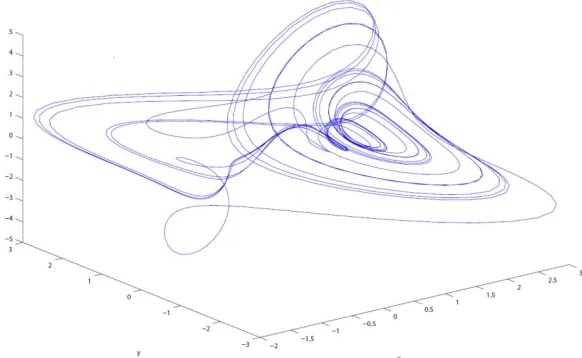
Interestingly, if the initial condition on capital is chosen in such a way that system S gives rise to a saddle-node bifurcation, then a continuum of equilibria can depart from a given initial condition of the predetermined variable, as clearly shown in Fig. 1, using the set of parameters in Chang et al. (2011).
Since this continuum of equilibria exists beyond the region relevant for the linear approximation of the dynamics in the neighborhood of the steady state, the result implies indeterminacy of global nature. Besides the result of global indeterminacy, the possibility that the model can exhibit this motion is of great interest also because the decomposition of the dynamics into phase/amplitude equations allows us to better understand the nature of the cyclical behavior of an economy where the effects of monetary policies on the long run properties of the equilibrium become totally unpredictable.
4. Concluding Remarks
In this paper we have extended the Chang et al. (2011) monetary policy model with an endogenous rate of time preference. We found that the equilibrium can be indeterminate under an active interest-rate feedback rule and the equilibrium is determinate (indeterminate) if the monetary authority implements an aggressively (moderately) passive interest-rate feedback rule. These results provide insightful policy implications by exploring the possibilities for the raise of global indeterminacy via a Shilnikov saddle-node bifurcation on an invariant circle. In this case, the economy may start at some point to oscillate around the long run equilibrium, and eventually deviate from its saddle-path stable solution, thus locating the economy in a particular optimal converging path that could not coincide with the one corresponding to the lowest desired interest rate.
5. Appendix
Consider a second order Taylor expansion of the vector field in (S):
1
3
( , , )
0
( , , )
f k
k f k
k
J
(A.1)
where 1 3 2
1( , , ) 2 ( 1)( 2)
f k k k and f3( , , )k ( 1)k 2k2
.
Assume now that system (S) undergoes a triple-zero eigenvalue structure, which allows us to make the following change of coordinates
1 2 3
w w w k
T
(A.2)
1 1 1
2 2
3
0
1 0
u v z
u v z
T (A.3)
whose columns represent the eigenvectors associated to the triple-zero eigenvalues (see, Wiggins, 1991).
We are thus able to put (A.2) in a Jordan normal form
1 1 2 3,
1 1
2 2 2 1 2 3,
3 3 3 1 2 3,
, ,
0 1 0
0 0 1 , ,
0 0 0 , ,
F w w w
w w
w w F w w w
w w F w w w
(A.4) where:
2 2 3 1 2 1 2 1 3 32
1 2 3, 2 3 1 2 1 2 1 3 3
2
2 1 1 2 2 1 2 1 3 3
( )
1
, , ( )
( ) ( )
i
v z A v z A w z w
F w w w u z A u z A w z w
D
v A u v u v A w z w
(A.5)
with Dv z2 1u v z1 2 3u v z2 1 3, and
3 1
1 2 ( 1)( 2)
A k
and
2
2 ( 1)
A k
.
Let us repeat the same procedure of above, and introduce a second transformation matrix 2 0 1 0 0 0 0
B (A.6)
which allows us to put system (A.4) into the normal form suitable to describe the presence of one zero and a pair of pure imaginary eigenvalues
1 1 1
2 2 2
3 3 3
0 0
0 0
0 0 0
x x F
x x F
x x F
where F1B w1( 122z w w3 1 3z w32 32),
2 2 2
2 2( 1 2 3 1 3 3 3)
F B w z w w z w ,
2 2 2
3 3( 1 2 3 1 3 3 3)
F B w z w w z w ; and 1
1 D 2 3 1 2 1 2
B v z A v z A ,
1
2 D 2 3 1 2 1 2
B u z A u z A , 1
3 D 2 1 ( 1 2 2 1) 2
B v A u v u v A .
System (A.7) can be easily transformed into cylindrical coordinates
3 2
1 2 3
2 2 3 2
1 2 3 4
2 2
1 2 3
r a rz a r a rz
z b r b z b z b r z
c z c r c z
(A.8)
given x1rcos, x2 rsin , x3 z (see Wiggins, 1991).
Additionally, the truncated-amplitude rescaled normal form can be derived from (A.8), keeping :
2 2
ˆ
ˆ
r arz
z br z
(A.9)
where 1
2
ˆ ab
a and bˆ 1.
A candidate for versal deformation of (A.9) is then
1
2 2
2
ˆ
ˆ
r r arz
z br z
(A.10)
References
Benhabib, J., S. Schmitt-Grohé and M. Uribe (2001) Monetary Policy and Multiple Equilibria American Economic Review 91, 167-186.
Chang, W.Y., H.F. Tsai and J.J. Chang (2011) Endogenous time preference, interest-rate rules, and indeterminacy Japanese Economic Review 62, 348-364.
Dupor, B. (2001) Investment and Interest Rate Policy Journal of Economic Theory 98, 85-113.
Mattana, P., K. Nishimura and T. Shigoka (2009) Homoclinic bifurcation and global indeterminacy of equilibrium in a two-sector endogenous growth model International Journal of Economic Theory 5, 1-23.