1
RSI RANGE DETERMINATION USING CUBICAL DISTANCE
CLASSIFICATION
Dr. A. CLEMENTKING ,S. SASIKALA
Faculty , Salalah College of Technology , Salalah , SULTANATE OF OMAN , Asst.Prof. in Computer Science , IDE , University of Madras,Chennai-5, INDIA,
E-mail : [email protected] , [email protected]
ABSTRACT
Information processing and decision support system using data mining techniques is in advance drive for huge availability of remote sensing image (RSI). RSI describe inbuilt properties of objects by recording their supernatural reflectance in the electro-magnetic spectral (ems) region. Information on such objects could be gathered by their color properties or their spectral values in each ems range of pixels Present paper explains a method of such information extraction using cubical distance methods and the results are discussed. This method is one among the simpler in its approach and considers grouping of equal distance of similar from a specified point in the image or selected pixel based on its attributes. The color distance and the occurrence pixel distance are played vital role to determine the similar distance objects in the RSI.
Key works : Cubical Distance Method, FIS, Color Map
1.0 INTRODUCTION
The objective of the present research process is to mine the digital values of selected RSI image with possible classification of pixels determining features and predicates the possible integration of applications using cubical distance method.. The classification process is implemented with the processed image digital values distance using classification and clustering algorithm with data mining techniques.
Remote Sensing is the science and art of acquiring information (spectral, spatial, and temporal) about material objects, area, or phenomenon, without coming into physical contact with the objects, or area, or phenomenon under investigation. Without direct contact, some means of transferring information through space must be utilized. In remote sensing, information transfer is accomplished by use of electromagnetic radiation (EMR). EMR is a form of energy that reveals its presence by the observable effects it produces when it strikes the matter. The Electro-Magnetic Radiation (EMR), which is reflected or emitted from an object, is the usual source of Remote Sensing data. However, any medium, such as gravity or magnetic fields, can be used in remote sensing. This represented in the combination of pixels and stored in the digital media for analysis and predications.
2.0METHODOLOGY
The following procedure is followed in this paper i.Capture satellite Image
ii.Preprocess the image using RSI tools and extract the RSI to process the image
iii.Convert the integrated multi layer image into two dimensional Digital number (DN) layer values
iv.Convert the multi layer image into two dimensional matrix using micro array
v.Determine the distance of the pixel using cubical distance determination methods a. From the origin (0,0,0)\
b. From the first point of the Region of Interest c. From the frequent occurrence point in the ROI
vi.Classification of Pixels according to the cubical distance
vii.Analysis the result
3.0 PREPROCESSING OF RSI
2 should be as straightforward as possible. We wish to maintain the characteristics of the data as it arrived from ERDAS IMAGIN 8.7 and use methods that require no special data (i.e. in situ atmospheric measurements). We believe this approach will help make the proposed cubical distance method more generally applicable and accessible to a wider group of possible users by using readily available satellite data and standard preprocessing algorithms.
3.1 Geometric Correction
The generally accepted procedure for geometric registration is to match a set of points on one image to those on the other. The coordinates from this set of points are then used to calculate a transformation function that will change the coordinates of one image so it will more closely match, geometrically, the other image. This is referred to as ground control point (GCP) registration. It is the registration method recommended by the NOAA C-CAP program (Dobson, et al., 1995). Our image-to-image registration was done within Imagine™ software using the “GCP Editor” (ground control point editor).
3.2 Radiometric Correction
In this section, The digital numbers to reflectance values using the sensor bias and gain calibration constants .The basic idea behind a radiometric correction is for differences in image data to represent actual differences in ground cover and not differences in atmospheric conditions and/or differences in the sensor. There are many methods that can be use to conduct radiometric normalization. Two general classes for these methods are 1) correction based on modeling the physical environment and 2) corrections using empirical adjustments based on scene comparisons. Empirical methods use only the image data and normalize one scene to another (Morisette et al., 1996). Corrections based on physical modeling used in the radiative transfer model
4.0 PIXELS TOWARDS OBJECTS
The strong motivation to develop techniques for the extraction of image objects stems from the fact that most image data exhibit characteristic texture which is neglected in common classifications. The texture of an object can be defined in terms of its smoothness or its coarseness. The image objects are constructed with combinational pixel standards of an object. These systems are used to assess characteristics of products by measuring the texture of their surface. In many cases, image analysis leads to meaningful objects only when the image is segmented into ‘homogeneous’ areas (Gorte 1998, Molenaar 1998, Baatz & Schäpe 2000, Blaschke et al. 2000). Segmentation is not new (see Haralick et al. 1973), but it is yet seldom used in image processing of remotely sensed data. Kartikeyan et al. (1998: 1695) state: “Although there has been a lot of development in segmentation of grey tone images in this field and other fields, like robotic vision, there has been little progress in segmentation of color or multi-band imagery.” One reason is that the segmentation of an image into a given number of regions is a problem with a huge number of possible solutions. The pixels are combinational values. How the values are extracted and constructed is presented in the micro array formations process.
5.0 MICRO ARRAY
The image represented in the multi dimensional layer based Digital numbers. The DNs are represented according to the layer such as R.G,B & IR. The Image layers are from 1 to 4. The Image extracted with three layer with possible combination (1,2,3), 1,2,4) etc. This combinational array are represented in the same cubical array . this array are converted into to equaling array in two dimension with following attribute procedure ( X,Y, layer1 value , layer2 value, layer3 value) . The size of the array is equal to number of total pixels into 5 columns.
Layer 1
125 134 143 146 144 145 148 147 134 126 126 125 127 139 145 144 144 137 146 140 127 128 131 122
Layer 2
134 141 147 128 141 139 146 138 141 135 126 111 140 139 135 126 138 139 148 145 143 139 116 106
Layer 3
137 132 139 139 141 141 153 151 145 129 120 130 123 125 139 137 131 148 153 143 139 133 134 132
Constructed macro array
3
6.0 PROCEDURE FOR CUBICAL DISTANCE
METHOD
i.Collect the pre processed RSI with the process able Image.
ii.Convert the multilayer integrated image into the Digital values.
iii.convert the cubical values into two dimensional array ( Number of Pixel ,5)
Each row represents (X,Y,R,G,B) values iv.Calculate the distance from the following
options
a. From the origin o(X,Y,Z)
Cubical Dis O = sqrt ( ( 0-X0)2 +( 0-Y0)2 +(
0-Z0)2)
b. From the First Position of the Region of
Interest FP(X,Y,Z)
Cubical Dis FP = sqrt ( ( 0-XFP)2 +( 0-YFP)2
+( 0-ZFP)2)
c. From the Frequent Item set of the Region
of Interest FIS(X,Y,Z)
Cubical Dis FIS = sqrt ( ( 0-XFIS)2 +(
0-YFIS)2 +( 0-ZFIS)2)
{ Different possible distance for each item is determined using above specified formula) v.Collect the number of classification( NC)
aimed to process
vi.determine the minimum (Min) and maximum(Max) cubical distance among the pixels in each method
vii.Determine the difference dx = Max – Min viii.The Range R = dx / NC
ix.Fix the starting pixel value and End pixel vales for each classification based on the cubical distance
x.Process all cubical distance rage. According to the individual and referral position of the pixel distance construct the classification data and sub image .
xi.Repeat the step 9 until all the classification to be processed for all the three methods . Display the result .
7.0 EXPERIMENT
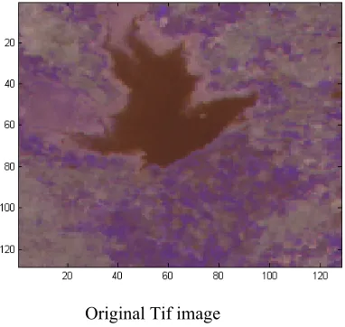
The preprocessed converted talk image selected for classification. The original.tif image selected for the process from (400,400) with the area of 381747 Sq.M2. The pixel value is equal to 23.3 meters. This
classification approach is manipulated based on the DNs of each layer together and each layer separately. The classified image and its range values of pixel based on cubical distance programme and executed using mat lab 7.0 are
presented below
Original Tif image
From the adopted ROI , the [400 x 400 , 5] pixel micro array constructed for the cubical distance calculated. The Frequent Item Set pixel determined using Integrated Development Algorithm[IDA] FIS algorithm. The cubical distance values are calculated suing above mentioned procedure. Based on the determined distance , the range values for each classification determined in each algorithm and determined the occurred pixel starting and end range vales. They are presented below with the percentage of occurred pixel in each classification. The execution done using matlab7.1a.
Analysis of Remote Sense Image
Name of the Image Original.tif
ROI Starting Points
(X,Y) 400,400 Number of Pixels
(X,Y) 128,128
Pixel: RSI Ratio 1:23.3 meters
Total Number of Pixel 16384
Total Area (Sq.M) 381747.2
Number of Cluster 8
4
Starting Range End Range
# of
Pixel % of Pixels
Class ifica
tion Red Green Blue Red Green Blue
F
rom
O
rig
in
(0,
0,0)
1 84 45 34 169 126 133 4290 26.18
2 No Classification
3 No Classification
4 84 45 34 92 47 33 129 0.79
5 84 49 41 114 60 49 641 3.91
6 92 53 102 134 81 69 4023 24.55
7 94 55 139 144 92 96 6196 37.82
8 105 63 178 160 95 129 1082 6.60
From t
he First
Pixel of R
O
I 1 84 45 34 169 126 133 4904 29.93
2 109 95 106 143 104 108 3853 23.52
3 101 82 107 153 105 115 3001 18.32
4 95 74 111 160 95 129 2401 14.65
5 92 57 96 163 121 133 1388 8.47
6 92 53 102 161 134 133 213 1.30
7 91 72 40 114 60 49 218 1.33
8 87 49 37 105 63 178 301 1.84
F
rom
FI
S of
RO
I
1 84 45 34 169 126 133 4290 26.18
2 No Classification
3 92 53 102 107 67 85 896 5.47
4 84 45 34 122 70 79 4560 27.83
5 89 46 33 136 81 90 3725 22.74
6 103 63 154 145 91 113 2239 13.67
7 105 63 178 159 90 119 584 3.56
8 143 125 120 161 118 129 82 0.50
5
The range value of cubical distance and classification represented in a form of graph
i) The classified images results of Starting Range and End Range for cubical distance from the origin(0,0,0) are presented below
S tarting R ang e Analys is of each C las s ification
0 50 100 150 200
C lusters/C lassifications
DN Va lu e s
R ed 84 84 84 92 94 105
G reen 45 45 49 53 55 63
B lue 34 34 41 102 139 178
1 2 3 4 5 6 7 8
E nd R ang e Analys is of E ach C las s ification
0 50 100 150 200
C lusters/C lassifications
DN Va lu e s
R ed 169 92 114 134 144 160
G reen 126 47 60 81 92 95
B lue 133 33 49 69 96 129
1 2 3 4 5 6 7 8
ii) The classified images results of Starting Range and End Range for the First Pixel of ROI FP(X,Y,Z)
are presented below
S tarting R ang e Analys is of eac h C las s ification
0 20 40 60 80 100 120
C lusters/C la ssifica tions
DN Va lu e s
R ed 84 109 101 95 92 92 91 87
G reen 45 95 82 74 57 53 72 49
B lue 34 106 107 111 96 102 40 37
1 2 3 4 5 6 7 8
E nd R ang e Analysis of E ach C lassification
0 50 100 150 200
C lusters/C lassifications
DN Va lu e s
R ed 169 143 153 160 163 161 114 105
Green 126 104 105 95 121 134 60 63
B lue 133 108 115 129 133 133 49 178
1 2 3 4 5 6 7 8
iii) The classified images results of Starting Range and End Range for the Frequent Item Set of ROI FIS(X,Y,Z) are presented below
S tarting R ang e Analys is of each C las s ification
0 50 100 150 200
C lusters/C lassifications
DN Va lu e s
R ed 84 92 84 89 103 105 143
G reen 45 53 45 46 63 63 125
B lue 34 102 34 33 154 178 120
1 2 3 4 5 6 7 8
E nd
Range
Analysis
of
E ach
C lassification
0 50 100 150 200 Clusters/Classifications DN Va lu e s
Red 169 107 122 136 145 159 161 Green 126 67 70 81 91 90 118 Blue 133 85 79 90 113 119 129
6
a. Result of sub images based on cubical distance from the origin(0,0,0)
1 4
7
7 8
b. Result of sub images based on cubical distance from the First Pixel of ROI FP(X,Y,Z)
1 2
8
5 6
7 8
c. Result of sub images based on cubical distance from the Frequent Item Set of ROI FIS(X,Y,Z)
1 3
9
6 7
8
8.0 INTERPRETATION
The above depicted images have represented the classified subimages of the cubical distance based on the distance from the origin (0,0,0), First point of the pixel of ROI and FIS of the Pixel of the selected ROI. In each layer, the object is identified in different class range. In each metod the classification occurrence, number of pixel and range varies one with another This is due to the varied distance values of the identified object in different spectral region of ems due to its inherent reflection and emission of the object in the particular area.
The following interpretations are derived from the observation of the analysis.
• In the cubical distance and the range values are not synchronized
• The object and the classification are not
similar one with another for each method
• Classification level, number of pixels and the range differs i.e the starting range and end range values vary with one another, which has been clearly brought out by the algorithm.
9.0 CONCLUSION
10
REFERENCES:
[1]. Breiman, L.: Bagging Predictors. Machine
Learning Vol. 26(2) 123–140, ( 1996)
[2]. Džeroski, S. (et al.): Using decision trees to predict forest stand height and canopy cover from LANSAT and LIDAR data. In:
Managing environmental knowledge:EnviroInfo 2006: proceedings of
the 20th InternationalConference on Informatics for Environmental Protection,Aachen: Shaker Verlag, pg.
125-133, (2006)
[3]. Efron, B. (et al.): An Introduction to the
Bootstrap. Chapman and Hall, New York, (1993)
[4]. Hyyppa, H. (et al.): Algorithms and Methods of Airborne Laser-Scanning for Forest Measurements. rnational Archives of Photogrammetry and Remote Sensing, Vol XXXVI, 8/W2, Freiburg, Germany, (2004)
[5]. Quinlan, J. R.: Learning with continuous
classes. In Proceedings of the 5th Australian Joint Conference on Artificial Intelligence, pages 343–348. World Scientific,Singapore, (1992).
[6]. Raymond, M. (et al.): Measures. Laser remote sensing: fundamentals and applications. Malabar, Fla., Krieger Pub. Co. 510 p. G70.6.M4 (1992)
[7]. SFS Slovenian Forestry Service: Slovenian
forest and forestry. Zavod za gozdove RS, 24 pp (1998)
[8]. Witten, I. (et al.): Data Mining: Practical
machine learning tools and techniques with Java implementations.Second Edition, Morgan Kaufman, (2005)
[9]. Clementking, A. Angel Latha Mary, S.
Comparing and identifying common factors in frequent item set algorithms in association rule 18-20 Dec. 2008 ISBN: 978-1-4244-3594-4- 10.1109/ICCCNET.2008.4787769. 2009-02-24.
[10]. Clementking, A. Angel Latha Mary, SStudy on Frequent Item set algorithms in association rule in International Journal of Algorithms, Computing and Mathematics Vol-1, NA.ov-1 2008 by Eashwar Publications
[11]. JANSSEN, L. (1993): Methodology for
updating terrain object data from remote