Efficient Mining Maximal Variant Usage and
Low Usage Biclusters in Discrete
Function-Resource Matrix
Lihua Zhang1,2, Miao Wang2,3,*, Zhengjun Zhai1, Guoqing Wang1,2,3
1School of Computer Science and Engineering, Northwestern Polytechnical University, Xi’an, China, 710072 2Science and Technology on Avionics Integration Laboratory, Shanghai, China, 200233
3China National Aeronautical Radio Electronics Research Institute, Shanghai, China, 200233 Email: {zhang_lihua, wang_miao,wang_guoqing}@careri.com
*Corresponding author
Abstract—The functional layer is the pillar of the whole prognostics and health management system. Its effectiveness is the core of system task effectives. In this paper, we proposed a new bicluster mining algorithm: DoCluster, to effectively mine all biclusters with maximal variant usage rate and low usage rate in the discrete function-resource matrix. In order to improve the mining efficiency, DoCluster
algorithm constructs a sample weighted graph firstly; secondly, all biclusters with maximal variant usage rate and low usage rate satisfying the variant usage rate and low usage rate definition are mined using sample-growth and depth-first method in the constructed weighted graph.
DoCluster algorithm also uses several pruning strategies to ensure the mining of maximal bicluster without candidate maintenance. The experimental results show DoCluster
algorithm is more efficient than other two algorithms.
Index Terms—bicluster, variant usage rate, low usage rate, function, resource
I. INTRODUCTION
The function is the foundation of task realization and also the basis of improving and guaranteeing quality, performance and effectiveness of system task information. The functional layer is the pillar of the whole system. Its effectiveness is the core of system task effectives. The health of the functional layer includes the status of functional components in the hierarchy range and overall health status of the whole functional layer. Health management objective of the functional layer is the effectiveness of the functional components and the hierarchy and to form function self-organizing platform based on the effectives of functional components. Although studying the effectiveness degree of resources is the base to construct a prediction and health management system [1]. The health degree of resources directly influences functional health. So, analysis of the call relation between functions and resources can excavate the health relation between them so as to complete the functions through using healthy resources and improve the health degree of functions.
The call relation of functions and resources can be abstracted as a matrix. In other words, each row means a resource and each column means a function, the value in the matrix is the use degree of a function to a resource. This value is defined during functional design, i.e. resource dependence degree of this function in aircraft system in order to complete a function. For example, for the resource whose storage spaces are 100K, function F1 needs 60K storage spaces to store some temporary variables. The dependence degree of this function on this storage resource is 0.6. Through mining the above function-resource matrix, the usage relation between a group of functions and a group of resources can be gained. For instance, for a group of functions F1F2F3, the resource relations called by each function are as follows:
F1==>R1R2R3, F2==>R2R4R5 and F3==>R6R7. Suppose
F1F2F3need to cooperate to complete a task T. All above three functions may be called at the same time. For resource R2, it supports F1 and F2 simultaneously. There may have two conditions: (1) R2 has high effectiveness for F1, but has low effectiveness for F2; (2) R2 has high effectiveness for both F1 and F2. The health degree of the first condition is higher than that of the second one. The reason is that, resource R2 can serve F1 and F2 simultaneously in the first condition; while in the second condition, resource R2 needs to serve for two functions. From the perspective of functional health, if resource R2 has defects, its influence on the first condition is lower than the second one. So, through function-resource matrix mining, in order to achieve a group of functions, the resources which can satisfy all functional demands simultaneously and the resources which can satisfy all functional demands through multiple accesses can be mined, i.e. mine bicluster with variant usage rate or low usage rate from function-resource matrix.
bicluster with variant usage rate and low usage rate described above from function-resource matrix. Currently, large quantities of algorithms based on greedy strategy or exploratory strategy are applied in mining bicluster. Cheng and Church proposed an algorithm based on greedy strategy [2]. This algorithm adopts a low square root residue to delete redundant nodes step by step. After that, many algorithms based on greedy strategy were raised [10-17]. All the above algorithms adopt the following two mining strategies: 1) produce cluster overall according to traditional clustering method and then optimize gradually; 2) mine bicluster in two types of data respectively and then gain the result through comparison and integration. But for the above two strategies, the efficiency of algorithms are not well. Thus, to design a high-efficiency bicluster mining algorithm is current research hotspot. So, Wang et al. came up with the mining algorithm to mine the maximal bicluster in discretized data [18].
The existing differential bicluster mining methods can be classified into two groups. One is to construct a difference matrix to mine discriminative biclusters. [19] developed a methodology for differential co-expression on a global scale. [20] proposed an algorithm to extract differential biclusters from the two gene expression datasets. [21] aims to mine subspace differential co-expression patterns. And it can also be used for mining differential biclusters. Another recent proposed algorithm called DeBi [22] uses frequent pattern mining approach
for discovering maximum size homogeneous bicluster in which all genes are co-expressed under a subset of samples. However, this algorithm cannot effectively mine bicluster with variant usage rate meeting difference restraint from function-resource matrix.
We can see through the above analysis that existing bicluster algorithm has some shortcomings during mining a bicluster with variant usage rate and with low usage rate. In order to improve mining efficiency, this paper proposed a new bicluster mining algorithm - DoCluster
algorithm which can effectively mine all biclusters with maximal variant usage rate and low usage rate from discrete function-resource matrix. Since the number of functions is far lower than that of resources in function-resource matrix, this algorithm uses sample-growth method for mining. First, a sample weighted graph is constructed, which includes all resource collections between both samples that satisfy the definition of variant usage rate or low usage rate; then, all biclusters with maximal variant usage rate and low usage rate satisfying the definition are mined with the mining method of using depth-first sample-growth method in the weighted graph. To improve the mining efficiency of the algorithm,
DoCluster algorithm uses several pruning strategies to
ensure the mining of maximal bicluster without candidate maintenance.
II. PROBLEM DESCRIPTION
Function-resource matrix is defined as a two-dimensional real matrix D= ×R F, in which row set R
represents the set of resources and column set F refers to
the set of functions. Element Dij of matrix D is a real number which represents the ability validity or usage rate of resource i supporting function j. |R| is the number of
resources in data set D and |F| is the number of functions
in data set D. For the convenience of mining, the original
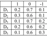
effective values in function-resource matrix are usually dispersed as 1, -1 and 0, where -1 means the usage rate of the resource is the minimum during the implementation of some function; 0 means the usage rate of the resource is moderate during the implementation of some function; 1 means the usage rate of the resource is the maximal during the implementation of some function, as shown in Table 1.
The significance of bicluster to be mined from function-resource matrix as shown in Table 1 is to mine a group of functions executed; under this group of functions, the usage rate of the resource is the maximal, i.e. which resources can reach the maximal usage rate when used together. In other words, the resources have the highest effectives when all functions are executed. For example, for a group of functions F1F2 (F1==>R1R2R3,
F2==>R2R4), these three functions may be called simultaneously. For resource R2, there are three situations for supporting F1 and F2: (1) for F1, the usage rate of R2 is high, while it is low for F1, as shown in Table 2; (2) for both F1 and F2, the usage rate of R2 is high, as shown in Table 3; (3) for both F1 and F2, the usage rate of R2 is low, as shown in Table 4, the health degree in the first and the third conditions is higher than the second condition. The reason is that R2 can serve F1 and F2 at the same time in the first and the third conditions resource. In the third condition, resource R2 needs to serve the two functions respectively. This paper puts forward that bicluster mined by DoCluster algorithm aims at the first and third
conditions.
TABLE I.
AN EXAMPLE OF FUNCTION-RESOURCE MATRIX
F1 F2 F3 F4 F5
R1 1 -1 -1 -1 1
R2 -1 1 -1 -1 1
R3 1 -1 -1 -1 0
R4 0 1 -1 -1 1
TABLE II.
AN EXAMPLE OF VARIANT USAGE RATE
F1 F2
R1 1 -1
R2 1 -1
R3 1 0
R4 0 -1
TABLE III.
AN EXAMPLE OF NON-VARIANT USAGE RATE
F1 F2
R1 1 -1
R2 1 1
R3 1 0
TABLE IV.
AN EXAMPLE OF LOW USAGE RATE
F1 F2
R1 1 -1
R2 -1 -1
R3 1 0
R4 0 -1
Definition 1. In order to facilitate description of bicluster with variant usage rate and low usage rate, suppose the use values of resource R1after discretization under the functions F1 and F2 are V1 and V2. There are four representations for R1 under F1 and F2: (1) if V1=1 and V2=-1, or V1=-1 and V2=1, the contribution rate of R1 to F1 and F2 satisfies diversity requirement, expressed as ‘R1’ and ‘*R1’ respectively; (2) if V1=-1 and V2=-1, the contribution rate of R1 to F1 and F2 satisfies diversity requirement, expressed as ‘-R1’; (3) if V1=1 and V2=1, the contribution rate of R1 to F1 and F2 does not satisfy diversity requirement, so no record is given; (4) if V1=0 or V2=0, the contribution rate of R1 to F1 and F2 does not meet diversity requirement, so no record is given.
Thus, in bicluster mined by DoCluster algorithm, each
resource can satisfy the first or the second conditions described above under all functions. To improve mining efficiency of the algorithm, DoCluster algorithm mines
biclusters with maximal variant usage rate and maximal low usage rate by using sample-growth method without candidate maintenance. The mining process of this algorithm will be introduced in the next section.
III. THE DOCLUSTER ALGORITHM
The mining steps of DoCluster algorithm can be
divided into two steps: firstly, scan original function-resource matrix, according to the definition of biclusters with maximal variant usage rate and maximal low usage rate, all sample weighted graphs satisfying the above definition are produced; then, use sample-growth method to mine all biclusters with maximal variant usage rate bicluster and maximal low usage rate bicluster.
A. Construct Sample Relational Weighted Graph
The method of mining modes with sample relational weighted graph was used in MicroCluster algorithm [12]
to mine bicluster firstly. Then, Wang et al. [18, 23] also used sample relational weighted graph to mine bicluster and fault-tolerant bicluster. DoCluster algorithm in this
paper will adopt undirected sample relational weighted graph (hereinafter referred to as sample weighted graph) to mine biclusters with maximal variant usage rate and maximal low usage rate.
Definition 2. Sample weighted graph can be expressed with the set G={ , , }E V W . Each node in the vertex set V
in the weighted graph represents a function. If an edge exists between a pair of vertices, this means the resource with variant usage rate or low usage rate exists below two functions represented by this pair of vertices. The set of the edges is denoted as E. The weights of each edge are
the resource set satisfying the definition of variant usage rate or the definition of low usage rate under the two
functions connected with this edge. The set of the weights is denoted as W.
According to the description in Definition 1, when the resources among functions satisfy the definition of variant usage rate, the weight between two functions does not satisfy commutativity. For instance, the weight under
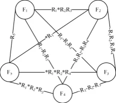
F1F2 is R1*R2R3, while the weight under F2F1 is *R1R2*R3. So, in Definition 2, the weight of each edge is the weight under FiFj, where i<j. Fig.1 shows the weighted graph corresponding to Table 1. For the convenience of follow-up description, Fig.2 provides storage structure of Fig.1.
R1 -R
2R
3
R 1-R
2R 3
R5
-R1R
2
-R3R
4
-R
1R 2-R 3R
4
Figure 1. The sample weighted graph constructed from Table 1
F1 R1*R2R3F2 R1-R2R3F3 R1-R2R3F4
F4 -R1R2-R3R4 F3
-R1R2-R3R4 F2
F4 -R1-R2-R3-R4 F3
F5 R2
F5 *R1
F5 *R1*R2*R4
F5 *R1*R2*R4 F4
Figure 2. The storage structure of Fig.1
B. Mining Maximal Bicluster
After the sample weighted graph is constructed, this section will introduce how DoCluster algorithm mines all
biclusters with maximal variant usage rate and maximal low usage rate from sample weighted graph without candidate maintenance in detail. According to the description in Definition 2, biclusters with variant usage rate and low usage rate extended satisfy anti-monotonicity, i.e. if the bicluster obtained by extension of
F1F2…Fn does not satisfy constraint conditions, neither does any superset F1F2…FnFm. Therefore, biclusters with a greater scale can be obtained by extension of the weight on each edge in the weighted graph in terms of intersection. But the bicluster mined by DoCluster is
different from the extension mode described in [18]. In
FDCluster algorithm, if S3 is gained through extending
S1S2, S1S2S3 set can be obtained through calculating the intersection of the weight of S1S2 and the weight of S1S3. However, this scheme cannot be used in this algorithm. It is required to calculate the intersection of the edges of
simultaneously. For example, in Table 1, for resource R2, when extended to F5from F1F2F3F4, R2is included in the weights under F1F5. However, R2 is not included in the weights under F2F5. If the intersection of R2 and the weight of F2F5 is not calculated when extended to F5 from F1F2F3F4, a wrong F1F2F3F4F5 bicluster including
R2 will emerge. So, when a new function is introduced in bicluster, it is necessary to calculate the intersection of all edges of the function newly introduced and the resource collection of bicluster extended. When calculating the intersection of the weights, it is only necessary to calculate the intersection of the resources, not necessary to consider ‘*’ or ‘-’ symbols before resources. With different symbols before resources, the intersection can also be calculated. These symbols are only used in pruning design.
We will introduce how DoCluster algorithm uses
pruning strategies to mine all biclusters with maximal variant usage rate and maximal low usage rate from sample relationship weight graph without candidate maintenance in detail. This paper will judge maximal bicluster with the method of backward checking proposed in [24] without candidate maintenance. That is to say, if resources under the current candidate sample and some prior candidate sample (mined sample) have some inclusion relation, i.e. all biclusters produced by the current candidate sample can be produced by some prior candidate sample, the current candidate sample can be pruned. When calculating the intersection of the weights, it is just necessary to calculate the intersection of resources, and the intersection can also be calculated with different symbols before resources. But, in accordance with the description (1) in Definition 1, since resource expression forms of V1=1 and V2=-1 or V1=-1 and V2=1, resource expression forms under F1F2 and F2F1 may be different. For example, when mining F2, the candidate functions are F3(-R1R2-R3R4), F4(-R1R2-R3R4) and F5(*R1), and the prior candidate function is F1(*R1R2*R3). Since currently F2 is extended, F1 is its prior candidate function. At this moment, F2F1(*R1R2*R3) should be produced, instead of F1F2(R1*R2R3). As resource expression forms under F1F2 and F2F1 are different, the weighted graph made by this algorithm is a directed graph rather than undirected graph. For Fn and Fm, it is necessary to build edges on FnFm and FmFn respectively. For FnFm and FmFn, the difference of weights on the edge is the interchange of resource expression forms “R1” and “*R1”. Therefore, for saving the storage space, the storage of weight is only that of weight on FiFi+1 edge. The weight on Fi+1Fi edge can be calculated with FiFi+1. For instance, the storage structure of Table 1 is as shown in Fig.2. F2F1(*R1R2*R3) can be gained through “complementing” F1F2(R1*R2R3) (“Ri” and “*Ri” interchange, and “-Ri” remains unchanged).
During function extension, the resource “symbol” is not considered. But during candidate function pruning, it is necessary to judge according to resource symbols under the candidate functions. Here, resource symbols under the candidate functions are decided by candidate
functions at current layer and resource symbols of the weights on the edge of initial extension function. For example, according to the storage structure shown in Fig.2, assuming the bicluster extended currently is F2F3
(-R1R2-R3R4), its candidate functions are F4(-R1R2-R3R4) and F5(*R1); its prior candidate function is F1(*R1R2*R3). Resource (-R1R2-R3R4) under candidate function F4 is gained through calculating the intersection of the weights of edges F2F4, F3F4 and F2F3. The “symbol” of each resource is the resource “symbol” on the edge F2F4. Because function F2 is extended currently, resource symbols of candidate functions are decided by F2F4. Similarly, for prior candidate function F1 of F2F3, its resource is also gained through calculating the intersection of F1F2, F1F3 and F2F3. Its resource symbols are decided by resource symbols on F2F1.
TABLE V.
AN EXAMPLE OF PRUNING USED MATRIX
F1 F2 F3 F4 R1 1 -1 -1 -1 R2 -1 1 -1 -1 R3 1 -1 -1 -1
Resource R1 is respectively expressed as ‘R1’ and ‘*R1’ above when the form of expression of resources is illustrated, just for the convenience of design of pruning strategies. For example, assuming there is the sole resource R1in Table 5, for R1, when the extension starts from F1F2, according to the above description, the expression form of R1 is ‘R1’. Assuming all functions extended from F1F2have been extended, when extending
F1F3, the expression form of R1 on the edge of F1F3 is also ‘R1’. At this moment, F1F3 can be pruned. It is known from the expression form of R1 that ‘1’ must exist under F1. According to previous variance definition, ‘1’ impossibly exists under other functions extended from F1. That is to say, R1 can only be ‘-1’ under F3. Therefore, functions which F1F3can extend must be gained through
F1F2extension. Meanwhile, F1F2can extend F3. So, F1F3 can be pruned.
If a resource in the current candidate function to be extended meets the form of ‘R1’, this resource can be pruned according to the Lemma 1 below.
Lemma 1. Assuming that P is the bicluster with
variant usage rate to be extended currently; M is the
candidate function set of P and N is the prior candidate
function set of P. If the expression form is ‘Rj’ for any resource Rj in candidate function Mi (Mi∈M) and there is a prior candidate function Nj (Nj∈N) under which resource Rj also exists, resource Rj in Mi can be obtained by extension of prior candidate function Nj.
Proof. Proof by contradiction is adopted. Resource expression form of current candidate function Miis ‘Rj’; a prior candidate function Nj (Nj∈N) exists; resource Rj also exists under Nj. Thus, Mican be pruned. In line with description (1) in Definition 1, for resource Rj, ‘1’ is under some function in P. In accordance with the
resource Rj must be ‘-1’ under candidate function Miand prior candidate function Nj. So, the bicluster extended currently must be a bicluster with variant usage rate. As only one ‘1’ can exist for each resource under all functions in the bicluster with variant usage rate, the bicluster with variant usage rate gained through extension of PMi can be obtained through extension of PNjMi. Thus,
Mi can be pruned. This contradicts the assumption, so the original proof is established.
However, for the expression form of ‘*’, the above pruning strategy is not applicable. For example, assuming there is the sole resource R2in Table 5, for R2, when the extension starts from F1F2, according to the previous description, the expression form of R2is ‘*R2’. Assuming all functions extended from F1F2 have been extended, when extending F1F3, the expression form of R2 on the edge of F1F3 is also ‘-R2’. At this moment, F1F3 can not be pruned. It is known from the expression form of R2 that ‘1’ must exist under F2. According to previous variance definition, ‘1’ likely exists under other functions extended from F1. That is to say, ‘1’ likely appears under the functions extended by F1F3. For R2, F1F3F4F5 can be gained through extension of F1F3, but F1F2F3F4F5 cannot be gained through extension of F1F2.Therefore, functions which F1F3can extend may not be gained through F1F2 extension. So, For R2, F1F3can not be pruned.
According to the above analysis, if a resource in the current candidate function to be extended satisfies the form of ‘*R1’, it should be judged whether this resource can be pruned according to the weight of prior candidate function. Therefore, the following Lemma can be used for pruning.
Lemma 2: assuming that P is the bicluster with variant
usage rate to be extended currently; M is the candidate
function set of P and N is the prior candidate function set
of P. If the expression form is ‘*Rj’ for any resource Rj in candidate function Mi (Mi∈M) and there is a prior candidate function Nj (Nj∈N) under which resource Rj with the expression form of ‘-Rj’ also exists, resource Rj in Mi can be obtained by extension of prior candidate function Nj.
Proof: Proof by contradiction is adopted. When resource expression form of current candidate function Mi is ‘Rj’; a prior candidate function Nj (Nj∈N) exists; resource Rjalso exists under Nj with the expression form of ‘-Rj’, Mican be pruned. In line with description (1) in Definition 1, for resource Rj, ‘1’ is under current candidate function in Mi. In accordance with the definitions of variant usage rate and low usage rate, resource Rj under all functions in P must be ‘1’. Since resource Rj also exists under Nj with the expression form of ‘-Rj’, the bicluster extended currently must be a bicluster with low usage rate. As only one 1 can exist for each resource in the bicluster with variant usage rate, the bicluster PNjMi with variant usage rate can be gained through extension of PNj. Thus, the bicluster with variant usage rate gained through extension of PMi can be obtained through extension of PNjMi. Thus, Mi can be
pruned. This contradicts the assumption, so the original proof is established.
Similarly, if a resource in the current candidate function to be extended meets the form of ‘-R1’, it should be judged whether this resource can be pruned according to the weight of prior candidate function. Therefore, the following Lemma can be used for pruning.
Lemma 3: assuming that P is the bicluster with variant
usage rate to be extended currently; M is the candidate
function set of P and N is the prior candidate function set
of P. If the expression form is ‘-Rj’ for any resource Rj in candidate function Mi (Mi∈M) and there is a prior candidate function Nj (Nj∈N) under which resource Rj with the expression form of ‘-Rj’ also exists, resource Rj in Mi can be obtained by extension of prior candidate function Nj.
Proof: Proof by contradiction is adopted. When resource expression form of current candidate function Mi is ‘Rj’; a prior candidate function Nj (Nj∈N) exists; resource Rjalso exists under Nj with the expression form of ‘-Rj’, Mican be pruned. In line with description (1) in Definition 1, for resource Rj, ‘-1’ is under current candidate function in Mi. In accordance with the definitions of variant usage rate and low usage rate, resource Rj under all functions of in P may be ‘-1’ or ‘1’ under some functions. Since resource Rj also exists under
Nj with the expression form of ‘-Rj’, the bicluster extended currently may be a bicluster with low usage rate or a bicluster with variant usage rate. As the expression form of resource Rj under current candidate function Mi is ‘-1’, the bicluster PNjMi with variant usage rate or low usage rate can be gained through extension of PNj. Thus, the bicluster with variant usage rate gained through extension of PMi can be obtained through extension of
PNjMi. Thus, Mi can be pruned. This contradicts the assumption, so the original proof is established.
Lemma 4: assuming that P is the bicluster with variant
usage rate to be extended currently; M is the candidate
function set of P and N is the prior candidate function set
of P. If the same prior candidate function Nj(Nj∈N) exists for each resource Rj in candidate function Mi(Mi∈
M), making each resource Rj in candidate function Mi meet the conditions in Lemma 1 or 2 or 3, candidate function Mi can be pruned.
Proof: the process of proof can be gained through merging the processes of proof in Lemma 1, 2 and 3, so it is omitted here.
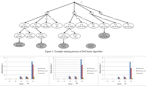
DoCluster algorithm deeply mines according to function
extension.
(1) Firstly, the extension starts from F1F2, and all candidate functions of F1F2 are produced: F3(R1-R2R3) and F4(R1-R2R3). The resource conditions after the intersection is calculated are shown in the brackets. When candidate functions are produced, the resource set under candidate function F3 of F1F2 can be gained only after the intersection of the weights of F1F2, F1F3 and F2F3 currently extended is calculated. Then, the candidate function F4(R1-R2R3) is produced through mining
F1F2F3(R1-R2R3). Here, when producing the resource set under candidate function F4, since the intersection of
F1F2F3 and F1F2F4 has been worked out, it can be obtained through calculating the intersection of the weights of F1F2F3, F1F2F4 and F3F4, without the need of calculating the intersection of each edge. So, the maximal bicluster F1F2F3F4(R1-R2R3) can be gained through extending F1F2 deeply and preferentially. Then, prepare to extend F1F2F4(R1-R2R3). For F1F2, when all resources in current candidate function meet pruning conditions in Lemma 1, 2 or 3 for prior F3. Therefore, F1F2F4can be pruned according to Lemma 4.
(2) Next, branch F1F3 is produced. All candidate functions of F1F3(R1-R2R3) are F4(R1-R2R3) and F5(R2). For F4, a prior candidate function F2(R1*R2R3) of F1F3 can be found. All resources of F4(R1-R2R3) are the subset of resources in F2(R1*R2R3), but resource R2 does not meet pruning conditions (Lemma 3). So, F1F3F4 can continue to be extended, but cannot be outputted. Then, the candidate function F5(R2) is generated through extending F1F3F4(R1-R2R3). Since F5(R2) does not meet pruning conditions, F1F3F4F5(R2) can be outputted. When preparing to extend F1F3F5(R2), since a prior F4 makes
F5(R2) satisfy the pruning conditions in Lemma 1,
F1F3F5(R2) should be pruned. Similarly, the branches of
F2, F3 and F4 can be mined respectively.
(3) When F2 is mined, its candidate functions are F3
(-R1R2-R3R4), F4(-R1R2-R3R4) and F5(*R1); its prior candidate function is F1(*R1R2*R3). As resources under
F2F3(-R1R2-R3R4) do not satisfy pruning conditions, it is necessary to continue to extend F2F3(-R1R2-R3R4) whose candidate functions are F4(-R1R2-R3R4) and F5(*R1) and prior candidate function is F1(*R1R2*R3). The candidate function F4(-R1R2-R3R4) dissatisfies pruning conditions, so it is necessary to continue extending to generate
F2F3F4(-R1R2-R3R4). The candidate function is F5(*R1) and the prior candidate function is F1(*R1R2*R3). Then,
F2F3F4F5(*R1) can continue to be generated and
outputted. According to pruning conditions, F2F4 and
F2F5 can be pruned.
(4) When extending to F3, the candidate functions of F3 are produced: F4(-R1-R2-R3-R4) and F5(*R1*R2*R4). Its prior candidate functions are F1(*R1-R2*R3) and F2
(-R1*R2-R3*R4). As resources in F4(-R1-R2-R3-R4) are the subset in prior candidate function F2(-R1*R2-R3*R4),
F3F4(-R1-R2-R3-R4) cannot be outputted. But F3F4(-R1-R2
-R3-R4) dissatisfies pruning conditions, so it is necessary to continue extending F3F4(-R1-R2-R3-R4) to produce the candidate function F5(*R1*R2*R4) and prior candidate functions: F1(*R1-R2*R3) and F2(-R1*R2-R3*R4). At this moment, F5 dissatisfies pruning conditions, so
F3F4F5(*R1*R2*R4) can be produced and outputted. For
F3F5(*R1*R2*R4), a prior F3F4(-R1-R2-R3-R4) exists, making F3F5 satisfy pruning conditions, so
F3F5(*R1*R2*R4) is pruned.
(5) When extending F4F5(*R1*R2*R4), a prior F4F3
(-R1-R2-R3-R4) exists, making F4F5 satisfy pruning conditions, so F4F5is pruned.
The above mining process is shown in Fig.3. The specific description of DoCluster algorithm is as follows:
Algorithm 1: DoCluster algorithm
Input: number threshold: rmin; function-resource matrix: D Output: all biclusters with maximal variant usage rate or maximal low usage rate meeting the threshold
Initial value: sample weight graph: G =Null, current
bicluster to be extended Q =Null, Si=Null and Sj=Null. Algorithm description: DoCluster(rmin, D, Q, Si, Sj) (1) If G is null, scan data set D and construct its
weighted graph. Si is the first sample in the weighted graph;
(2) For each sample Sj connected with sample Si
(3) If all resource linked lists in Sj satisfy pruning conditions in Lemma 4, then
(4) Continue; (5) Else
(6) For resource linked lists not satisfying pruning conditions, Q.Sample= Q.Sample∪Sj;
Q.Resource= Q.Resource∩SiSj.Resource; (7) DoCluster(rmin, D, Q, Si, Sj->next); (8) Endif
(9) Endfor
(10) If Q satisfies maximal definition, then
(11) Output Q
Figure 3. Example mining process of DoCluster algorithm
Figure 3. The comparison of performance periods of the above three algorithms under each data set when the number of functions is 20: (a) 200 resources;(b) 500 resources;(c) 800 resources
Figure 4. The comparison of performance periods of the above three algorithms under each data set when the number of functions is 35: (a) 200 resources;(b) 500 resources;(c) 800 resources
Figure 5. The comparison of performance periods of the above three algorithms under each data set when the number of functions is 50: (a) 200 resources;(b) 500 resources
IV. EXPERIMENTAL RESULT AND ANALYSIS
In this section, we will make an experimental comparison on the mining efficiency and result of the algorithm above and existing algorithms. The hardware environment of the experiment is desktop computer: Intel(R) Core(TM)2 Duo 2.53GHz CPU and 4G memory; the software environment is Microsoft Windows 7 SP1
TABLE VI.
THE PROPORTION OF EACH VALUE IN FIVE DATA SET
1 0 -1 D1 0.2 0.7 0.1
D2 0.3 0.6 0.1
D3 0.1 0.7 0.2
D4 0.2 0.6 0.2
D5 0.1 0.6 0.3
In this section, the comparison will be made on the mining efficiency of DoCluster algorithm FDCluster_One algorithm and MMCluster algorithm. FDCluster_One algorithm adopts prior detection method
described in literature [18]: mine maximal bicluster from discretized matrix data without candidate maintenance. The mining process of MMCluster algorithm and FDCluster_One algorithm is basically the same. The
difference is that during design of pruning strategy,
MMCluster algorithm first judges whether the gene set of
current potential samples is the subset of a prior candidate sample set, while FDCluster_One algorithm first
calculates the intersection and then judges prior samples. The mining efficiency of the above three algorithms is compared as follows. To fully compare the scalability of algorithms, we produce multiple groups of data sets with different numbers of resources and functions in allusion to five data sets in Table 6. The selection of resources and functions are based on the order of resources and functions in data set. Figures 4(a)-4(c) provide the comparison of performance periods of the above three algorithms under each data set when the number of functions is 20 and the number of resources is 200, 500 and 800 respectively. It can be seen from these figures that the mining time of each algorithm increases progressively with the increase in the proportion of ‘-1’ in the data set. This is because the biclusters with variant usage rate and low usage rate do not restrain the number of ‘-1’. Thus, as the number of ‘-1’ increases in the data set, the scale of the bicluster mined will increase continuously, thus increasing mining complexity of each algorithm. It thus can be seen, for mining of function-resource matrix, the number proportion of ‘-1’ in the data set directly influences the complexly of the algorithm. But, when the proportion of ‘-1’ is certain, as the proportion of ‘1’ increases in the data set, the complexly of the algorithm also increases. For data sets D1 and D2, the three algorithms can complete mining within 0.5s. The efficiency superiority of DoCluster algorithm is not
obvious. However, as the proportion of ‘-1’ in the data set increases, in data sets D3, D4 and D5, the pruning strategy of DoCluster algorithm displays efficiency superiority.
To further test and verify the scalability of algorithms, figures 5(a)-5(c) provide the comparison of performance periods of the above three algorithms under each data set when the number of functions is 35 and the number of resources is 200, 500 and 800 respectively; figures 6(a)-6(c) provide the comparison of performance periods of the above three algorithms under each data set when the number of functions is 50 and the number of resources is 200 and 500, respectively. It can be seen from these figures that the mining efficiency of the three algorithms
declines significantly compared with Fig.4 with the increase in the number of functions. This is because the three algorithms adopt row extension for mining. As the number of samples in the data set increases, mining depth and complexity of the algorithms increase. Meanwhile, the number of prior candidate samples for pruning judgment will also increase, thus increasing pruning complexity. In most data sets shown in Fig.5 and 6, the mining efficiency of DoCluster algorithm is the highest.
However, in the data sets with large proportion of ‘1’,
DoCluster algorithm fails to show the advantage of
mining efficiency. This may be because multiple biclusters including ‘1’ can exist simultaneously in the biclusters mined by MMCluster algorithm and FDCluster_One algorithm, while at most one ‘1’ can be
included in a bicluster mined by DoCluster algorithm due
to the restraint of the bicluster with variant usage rate. So, the number of biclusters mined by DoCluster algorithm is
greater than the above two algorithms, thus including the pruning efficiency of the algorithm.
V. CONCLUSION
This paper proposed an efficient algorithm - DoCluster
algorithm which can effectively mine all biclusters with maximal variant usage rate and low usage rate from the discrete function-resource matrix. First, this algorithm constructs a sample weighted graph which includes all resource collections between both samples that satisfy the definition of variant usage rate or low usage rate; then, all biclusters with maximal variant usage rate and low usage rate meeting the definition are mined with the mining method of using sample-growth and depth-first method in the constructed weighted graph. To improve the mining efficiency of the algorithm, DoCluster algorithm uses
several pruning strategies to ensure mining maximal bicluster without candidate maintenance. However, original data information will be lost if the mining is conducted in discrete data. Our next research direction is to mine biclusters with variant usage rate and low usage rate in real function-resource matrix.
ACKNOWLEDGMENT
This paper is supported by National Key Basic Research Program of China under Grant No. 2014CB744900.
REFERENCES
[1] Michael Pecht,et al.. A prognostics and health management roadmap for information and electronics-rich systems. Microelectronics Reliability, 2010:317–323.
[2] Y. Cheng, G.M. Church, “Biclustering of Expression Data,” Proc. 8th Int’l Conf. Intelligent Systems for Molecular Biology (ISMB00), ACM Press, 2000, pp: 93– 103.
[3] Cui Xiang, Yin Guisheng, Zhang Long, Kang Yongjin. Method of Collaborative Filtering Based on Uncertain User Interests Cluster. Journal of computers, Vol 8, No 1, 2013, p:186-193.
MKmeans. Journal of computers, Vol 8, No 1, 2013, p:10-17.
[5] Olovnikov I, Le Thomas A, Aravin A A. A Framework for piRNA Cluster Manipulation. PIWI-Interacting RNAs. Humana Press, 2014: 47-58.
[6] Fotso H, Yang S, Hafermann H, et al. Extended Correlation in Strongly Correlated Systems, Beyond Dynamical Cluster Approximation. Bulletin of the American Physical Society, 2012, 57.
[7] Xiao Xue, Zhe Wei, Zhifeng Zeng. The Design of Service System for SMEs Collaborative Alliance: Cluster Supply Chain. Journal of Software, Vol 6, No 11, 2011, p:2146-2153.
[8] Ling-ling Pei, Zheng-xin Wang. An Optimized Grey Cluster Model for Evaluating Quality of Labor Force. Journal of Software, Vol 8, No 10, 2013, p:2489-2494. [9] Yu Wang, Youfang Huang, Huiqiang Zheng, Daofang
Chang. Quay Crane Allocation of Container Terminal Based on Cluster Analysis. Journal of Software, Vol 8, No 5, 2013, p:1201-1208.
[10]Ben, et al. Discovering local structure in gene expression data: the order-preserving submatrix problem. J. Comput. Biol, 2003; 10: 373-384.
[11]Cheng et al. Bivisu: software tool for bicluster detection and visualization. Bioinformatics, 2007, 23: 2342-2344. [12]Lizhuang Zhao, Mohammed J. Zaki, MicroCluster: An
Efficient Deterministic Biclustering Algorithm for Microarray Data, in IEEE Intelligent Systems, special issue on Data Mining for Bioinformatics, 2005, Vol. 20, No. 6, pp: 40-49.
[13]U. Maulik, A. Mukhopadhyay, M. Bhattacharyya, L. Kaderali, B. Brors, S. Bandyopadhyay, and R. Eils. Mining Quasi-Bicliques from HIV-1-Human Protein Interaction Network: A Multiobjective Biclustering Approach. IEEE-ACM Transactions on Computational Biology and Bioinformatics, vol.10, 2013, pp.423-435.
[14]de Sousa Filho G F, dos Anjos F Cabral L, Ochi L S, et al. Hybrid Metaheuristic for Bicluster Editing Problem. Electronic Notes in Discrete Mathematics, 2012, 39: 35-42. [15]Király A, Abonyi J, Laiho A, et al. Biclustering of
High-throughput Gene Expression Data with Bicluster Miner. Data Mining Workshops (ICDMW), 2012 IEEE 12th International Conference on. IEEE, 2012: 131-138.
[16]Desai B, Andhale P, Rege M, et al. Biclustering and feature selection techniques in bioinformatics. Data Engineering and Management. Springer Berlin Heidelberg, 2012: 280-287.
[17]Pio G, Ceci M, D'Elia D, et al. A novel biclustering algorithm for the discovery of meaningful biological correlations between miRNAs and mRNAs. EMBnet. journal, 2012, 18(A): pp. 43-44.
[18]Miao Wang, Xuequn Shang, Shaohua Zhang, Zhanhuai Li. FDCluster : Mining frequent closed discriminative bicluster without candidate maintenance in multiple microarray datasets. ICDM 2010 workshop on Biological Data Mining and its Applications in Healthcare, p 779-786. [19]Lucinda K. Southworth, Art B et al, Aging Mice Show a
Decreasing Correlation of Gene, PLoS Genetics, December 2009, Volume 5,Issue 12.
[20]O. Odibat, C. K. Reddy and C. N. Giroux. Differential biclustering for gene expression analysis. In Proceedings of the ACM Conference on Bioinformatics and Computational Biology (BCB), 2010, p: 275–284.
[21]G. Fang, R. Kuang, G. Pandey, M. Steinbach, Chad L. Myers and V. Kumar. Subspace Differential Coexpression Analysis: Problem Definition and A General Approach.
Proceedings of the 15th Pacific Symposium on Biocomputing(PSB), 2010, 15:145-156.
[22]A. Serin and M. Vingron. Debi: Discovering differentially expressed biclusters using a frequent itemset approach. Algorithms for Molecular Biology, vol. 6, no. 1, 2011, p:18-29.
[23]Miao Wang, Xuequn Shang, Miao Miao, Zhanhuai Li, Wenbin Liu. FTCluster: Efficient Mining Fault-Tolerant Biclusters in Microarray Dataset. Proceedings of ICDM 2011 workshop on Biological Data Mining and its Applications in Healthcare, p 1075-1082.
[24]Wang, J, Han, J. BIDE: Efficient Mining of Frequent Closed Sequences, Data Engineering, 2004. Proceedings. p: 79 – 90.
Lihua Zhang is a doctoral student at the
school of computer science and engineering at the northwestern polytechnical university, Xi'an China. She completed her master degree from northwestern polytechnical university in 2008. Her current research interests are PHM, avionics, data mining and safety. Since 2013, she has been studying at science and technology on avionics integration laboratory.
Miao Wang is an engineer at science
and technology on avionics integration laboratory. He completed his doctor and master degree from northwestern polytechnical university in 2013 and 2018, respectively. He is a member of China computer federation. His research interests mainly include data mining, PHM, avionics and safety.
Zhengjun Zhai is a professor at the
school of computer science and engineering at the northwestern polytechnical university, Xi'an China. He is vice chairman of NPU youth association for science and technology, distinguished expert of aerospace electrical & electronics and weapon system Standardization technology committee, distinguished expert of AAMRI and premium member of china computer federation. His research interests include experiment and testing systems Integration, remote maintenance and fault diagnosis and virtual visualization.
Guoqing Wang is a professor and a