Optimizing Data Distribution for Loops on
Embedded Multicore with Scratch-Pad Memory
Qiuyan Gao
a, Qingfeng Zhuge
b, Jun Zhang
a,b, Guanyu Zhu
d, and Edwin H.-M. Sha
b,c a College of Information Science and TechnologyHunan University, Changsha, China. b College of Computer Science
Chongqing University, Chongqing, China.
Email:{ angela.gao8908, qfzhuge, jeffjunzhang}@gmail.com c Department of Computer Science
University of Texas at Dallas, Richardson, Texas 75080, USA. Email: [email protected]
d Huawei Technologies Co. Ltd., Shenzhen, China.
Email: [email protected]
Abstract— Software-controlled Scratch-Pad Memory (SPM) is a desirable candidate for on-chip memory units in embedded multi-core systems due to its advantages of small die area and low power consumption. In particular, data placement on SPMs can be explicitly controlled by software. Therefore, the technique of data distribution on SPMs for multi-core system becomes critical in exploiting the advantages of SPM. Previous research efforts on data allocation did not consider the placement of array data accessed in loops. Loops are the most time-consuming and energy-consuming part for most of the computation-intensive applications. In this paper, we propose a high-performance, low-overhead data distribution technique, the Iterational Optimal Loop Data Distribution Algorithm based on dynamic programming. It optimizes data allocation of both scalar and array data for embedded multi-core systems with SPMs. The experimental results show that the IOLDD algorithm reduces the energy consumption by 30.12% and 14.52% on average compared with random data distribution and greedy stretagy, respectively. It also reduces the memory access time by 18.45% and 18.38% on average compared with the random distribution strategy and the greedy strategy, respectively.
Index Terms— Data distribution, multi-core, scratch-pad memory, embedded systems
I. INTRODUCTION
M
ULTI-CORE design becomes the mainstream of high-performance embedded systems because of the ever-increasing demand on performance for applica-tions such as digital signal processing, wireless communi-cation, and mobile computing. Meanwhile, the design of multi-core systems usually has to satisfy strict require-ments on low power consumption and small die area. Therefore, Scratch-Pad Memory becomes an effective design alternative to replace cache as on-chip memory in embedded multi-core systems. Software-controlled SPM guarantees a single-cycle access time with low energyconsumption and small die area compared with hardware-controlled cache. In particular, data on SPM can be precisely controlled by software during system design. Many digital signal processing systems such as Analog Devices ADSP-BF534/6/7 [1] and TI’s TMS370CX7X [2], as well as multicore architectures such as NVIDIA GeForce 8800 [3], employ SPM as on-chip memory [4]. Therefore, how to efficiently distribute data items to on-chip SPMs to minimize the memory access cost becomes one of the key problem for fully exploiting the advantages of SPMs in embedded multi-core systems.Because loops are the most time and energy consuming code section in most of the computation-intensive applications, it is desirable to have efficient techniques to allocate array data, as well as scalar data, to multiple SPMs in a multi-core system.
A lot of multi-core systems employs symmetric mul-tiprocessing (SMP) architecture. Multiple cores share a centralized main memory. Each core is equipped with a small and fast on-chip SPM to speed up data accesses. Usually, there is only one copy of each data item. Data items accessed by multiple cores can spread on SPMs for multiple cores. The cost for searching and moving data items around, however, is high for multicore systems. In this paper, we propose a technique for keeping and up-dating one copy of array data in main memory efficiently with a minimized backup cost. Furthermore, we propose a data duplication method to replicate local copies for read-only data to further reduce the data access cost.
In this paper, we make the following contributions:
1) We propose a polynomial-time data distribution algorithm, the Iterational Optimal Loop data Dis-tribution algorithm with Duplication (IOLDD), to minimize the total cost of memory access on multi-core systems equipped with SPMs for both arrays and scalar variables in loops.
2) We present a data duplication technique and in-tegrate it into the data distribution algorithm. It further reduces the total cost of memory accesses by replicating multiple copies for read-only data items.
The rest of this paper is organized as follows. Related works are discussed in Section II. Models and some basic concepts are introduced in Section III. A motivational example is discussed in Section IV to illustrate some basic ideas of our algorithm. The problem definitions used in the paper are given in Section V. In Section VI, details of our improved dynamic approach IOLDD are presented. Section VII presents our experiments and Section VIII concludes the whole paper and mentions the future work.
II. RELATEDWORKS
There are a lot of works tackling the data distribution problem. Some of the works proposed static data distribu-tion methods. The data distribudistribu-tion is determined for the whole program and will not change during the execution of the program [6] [7] [8]. The drawback of static methods is that it cannot explore the benefit of varying data locality in a running environment. The other category of previous techniques is dynamic data distribution [9] [10] [11]. For those dynamic methods, program will be divided into different regions. Data movement instructions are inserted before each region to generate data distribution for a program region. The data distribution remains the same in the execution of a particular region. Greedy strategy, for example, is used to find a data distribution for each region by Udayakumaran in [12] [13]. Since dynamic data distribution takes advantage of the data locality of each program region, they have better performance than the static ones.
Array data is different from scalar data. Elements in array occupy contiguous memory locations. A single iterative statement in loop may process arbitrarily many elements of an array. Distributing array data is, therefore, quite different from the way we handle scalar data. To the best of the authors’ knowledge, there is not much research work conducted on data distribution for arrays in a loop, and some methods greatly rely on the loop’s characteristics. O. Ozturk et al. proposed algorithms to manage data for array-intensive nested loops with regular data access patterns [14] [15]. R. Thakur et al. proposed efficient algorithms to manage dynamic redistribution of arrays [16]. W. Huan et al. proposed algorithms to optimize all of the data segments, including global data, heap and stack data in general [17]. These methods do not consider the case of distributing both array and scalar data items in a loop on multi-core systems.
Research efforts have also been taken on the data distribution problem for SPMs. R. Banakar et al. pro-posed a simple SPM data management algorithm. But the algorithm cannot guarantee to achieve optimal results and is only applicable to scalar data [4]. Jun Zhanget al. proposed an algorithm for loops on single-core systems instead of multi-cores [18]. Y. Guo and Q. Zhuge et al. proposed a polynomial-time algorithm to solve the data distribution problem on multiple types of memory units [19] [20]. However, they only consider distribution for scalar data items and do not mention data distribution for loops. The data distribution problem for array data is very important for most of the applications. In this paper, we focus on developing a dynamic programming approach for both array and scalar data items on multi-core systems.
III. MODELS ANDBASICCONCEPTS
In this section, we first introduce the hardware architec-ture. Then, we will present the program execution model we use in this paper.
A. Hardware Architecture
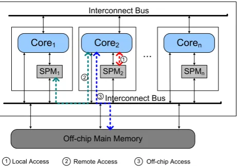
Figure 1. A multi-core hardware architecture.
The organization of on-chip memories of our hardware architecture is shown in Fig. 1. Every core has its own on-chip SPM, while all cores share the DRAM main memory. Each core can access its own local SPM. It can also access data items on other cores’ SPMs by the interconnect bus. Scratch-pad-memory here can be organized as a Virtually Shared SPM (VS-SPM) architecture for on-chip memory that takes advantage of both shared and local SPM [21]. Distinct from the local SPM, SPMs of other cores are referred to as remote SPMs. There is no limit for the number of remote SPMs that a core can access in the architecture.
longer latency than the local access. Objectively, for the low performance of DRAM and the high communication cost, latency of off-chip access is much longer than the latencies of both local and remote accesses [22]. In our architecture, each core can access all remote SPMs. Let Dist be the distance between two cores. The cost of remote access is a non-decreasing functionf of Dist.
B. Execution Model
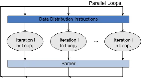
Figure 2. Demonstration of execution model for Loops .
In this paper, we consider the data distribution problem for loops can be paralleled in the program. A barrier is used to synchronize the execution of each iteration for all the loops. We also consider each basic block of a program as a program region. The execution model of loops executed in parallel on a multi-core system is shown in Fig. 2. Assume that there is no conditional branch in loop body. Each iteration is regarded as a program region by the compiler. The number of accesses on each data item in a program region can be obtained through profiling. Compiler inserts data distribution instructions at the beginning of a loop iteration. Therefore, data items are allocated to various memory units before parallel regions are executed. In case of conditional branch existing in loop body, each branch then should be considered as a program region. Data distribution instructions should be inserted at the beginning of each region. The data distribution problem considered in this paper tries to explore the opportunity of the optimal data placement on SPMs in multi-core systems. It aims to improve the performance and reduce the cost of memory accesses for our execution model.
IV. MOTIVATIONALEXAMPLE
In this section, a motivational example is presented to illustrate the main idea of the proposed algorithm (IOLDD). The goal of optimization is to minimize the total memory access cost of a parallel iteration in loops. In this motivational example, we assume all data items have the same size. Thus, the size of SPM is denoted by the number of data items that can be stored in SPM. Focus on the architecture shown in Fig. 1, we assume the system has only two cores Core1 andCore2. Each core
is equipped with an on-chip SPM marked asSP M1and SP M2, respectively. For the purpose of simplicity and
illustration, we assume thatSP M1has a capacity of two,
andSP M2 can hold three data items in the motivational
example. All cores can access the shared main memory, which is large enough to store all data items.
Figure 3. The loop programs forCore1andCore2 in the example Given two loop programs, as shown in Fig. 3,Loop1is
assigned toCore1andLoop2is assigned toCore2. There
are seven data items to be accessed: two scalar data items d1,d2 and five array data itemsA[i],A[i−1],A[i−2], A[i−3] and B[i]. Each data item can be assigned to SP M1 or SP M2. Besides, each iteration is regarded as
a program region, and in the execution model, the iteration in loop body forms a parallel region.
TABLE I.
NUMBERS OF DATA ACCESSES FOR EACH CORE
Data d1 d2 d3(A[i]) d4(A[i-1]) d5( A[i-2]) d6(A[i-3]) d7(B[i])
Core1Access 0 0 2 3 2 0 2
Core2Access 1 1 0 3 3 3 0
The number of seven data accesses in one iteration is shown in Table I. Both Core1 and Core2 can access
these data items and they run in parallel. The “Ac-cess” operation includes both “Read” and “Write” opera-tions for the core. In Table I, take Core1 for example,
row “Core1Access” shows the access times of Core1
for the data items. The corresponding loop program in Core1 is depicted in Fig. 3(a). For data d1, we know Core1Access(d1) = 0 and Core2Access(d1) = 1. In Loop1,Core1 has neither “Read” operation nor “Write”
operation for data d1. While in Loop2, data d1 is read
once. In this paper, we define a data which is “Read” by some cores and not “Written” by any core as a “Read-only” data. The problem of this example is how to find a data distribution for the seven data items in each iteration such that their total cost of memory access is minimized.
TABLE II.
NOTATIONS USED IN EXAMPLES
Notation Time (µs) Definition
Readspmi 1 the cost of reading fromCorei’s SPM.
Writespmi 1 the cost of writing toCorei’s SPM.
Readspmj→spmi 20 the cost of reading fromCorej’s SPM toCorei’s SPM.
Writespmj→spmi 20 the cost of writing fromCorej’s SPM toCorei’s SPM.
ReadM 60 the cost of reading from main memory.
WriteM 60 the cost of writing to main memory.
Migrationspmi→spmj 21 the cost of moving data fromCorei’s SPM toCorej’s SPM.
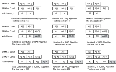
Figure 4. Costs and Distribution of each iteration with three different methods
remote SPM access cost function is a linear function f(d) = 20∗d. Since there are two cores in the system, the distancedequals 1. Therefore, the remote SPM accessing costsReadspmj→spmi andW ritespmj→spmi are 20.
We solve the problem with three strategies. One is the greedy strategy (Uday), which is derived from Udayaku-maran’s algorithm [12] [13] on single-core systems. The other is dynamic programming strategy on single-core (IDAS), which is derived from Zhang’s paper [18]. Fi-nally, it is our iterational optimal strategy (IOLDD), which will be presented in detail in Section VI.
The greedy algorithm is derived from Udayakumaran’s algorithm in [12] [13], and we call it “Uday” for short. The algorithm is a greedy algorithm, it distributes data items according to their read and write access times of all cores. However, the approach only targets single-core processors. For the purpose of comparison, we adopt the algorithm and apply it on multi-core systems.
The derived Uday algorithm works as follows: To begin with, data items are sorted according to their total number of accesses which is the sum of the number of accesses from all cores to this data. After that, data with the most total number of accesses is picked by the compiler. Then the compiler distributes the data into the available SPM of the core that accesses the data most times. When all the SPMs of the cores are full, the data should be distributed into the main memory.
As to the IDAS algorithm, it is derived from Zhang’s algorithm in [18]. Though the algorithm is a dynamic programming algorithm, it is limited in single-core sys-tems. Besides, it can not fully utilize the benefits of the private local SPM on each core. On the other side, the
IOLDD algorithm propose a duplication mechanism to utilize the distinct costs of data to/from local SPM, remote SPM and main memory. It is a technique that achieves higher time efficiency at the cost of space. In multi-core systems, traditionally, a data item has only one copy in either one of the SPMs or main memory. Multiple cores may access the same data in one parallel region. It is sometimes beneficial to duplicate data and place multiple copies of the same data in different SPMs. However, some of the data items cannot be duplicated because of high synchronization cost. Therefore, we only allow read-only data items to be duplicated.
TABLE III.
COSTCOMPARISON AMONG THREE DIFFERENT METHODS
Tech. Initial Data Distribution Iteration 1 Iteration 2 Cost Imprv. Cost Imprv. Cost Imprv.
IOLDD 599 — 456 — 456 —
Uday 755 20.66% 614 25.73% 614 25.73% IDAS 656 8.69% 496 8.06% 494 7.69 %
Results of the example with three strategies can be seen in both Table III and Fig. 4. The final data distribution for Uday algorithm results in a time cost of 614µs. To avoid array data items in loop being distributed in different SPMs and hard to find, we use the technique of update and have the backups of arrays in main memory. As shown in Fig. 4, these updated data items are distinguished by gray boxes. For IDAS algorithm, dataA[i−3]needs to be updated to main memory. Since dataB[i]has already been in main memory, it does not need to be updated. Time cost can finally be reduced to 494µs. For IOLDD algorithm, data A[i−1] is located in both SP M1 and SP M2, we say data A[i−1] is duplicated. The final
other two algorithms. Thus, we can conclude that IOLDD algorithm works better than both the Uday algorithm and IDAS algorithm in the motivational example.
V. PROBLEMDEFINITION
In this section, definitions for the problem of loop data distribution on multi-core systems are presented. Firstly, the following notations and definitions are used:
Notation Definition
D a set of distinct data items for loops {d1, d2, ..., dN}, where data can be either a scalar data or an array data item.
SP M a set of SPMs on each core
{spm1, spm2, ..., spmT}, where T is a constant. Besides,m0is the main memory.
Core a set of cores in hardware archi-tecture{Core1, Core2, ..., CoreT}. Each coreCoreihas its own on-chip local SPMspmi.
CAcci(dj) the number of access times for data
djby Corei.
distP(dj) a loop data distribution function for datadj defined fromD toSP M in one iterationP.
Costspmi(dj) a cost of memory access for datadj inspmi without duplication.
Costspmi+k+...(dj) a duplication cost of memory access for data dj where dj is in (spmi,
spmk, ...).
For function distP: D→SP M, ifdistP(d
j) = spmi, it indicates data dj is distributed to spmi on Corei in iteration P. Therefore, distP−1(d
j) represents the location of data dj before the execution of iteration P in loop body.
Loop Data Distribution Problem. Given a set of data items D in iteration P, a set of SPMs SP M. Sizespmi represents the capacity of spmi ∈ SP M,
Sizedj means the size of datadj. The loop data distribu-tion problem is to find a mapping between data dj ∈D and SPM spmi ∈ SP M. The total cost of memory access CostdistP(dj)(dj) is minimized, and inequality
∑
∀dj∈D,distP(dj)=spmiSizedj ≤Sizespmi is satisfied.
Definition 1: Migration Cost. The data migration cost is the cost of retrieving one data item from its original location and writing it to another memory unit. Hence, the migration cost is defined as the sum of one read operation from the original location and one write operation to the destination memory unit, as shown in Equation 1.
M igrate(dj) =
Readspmi+W riteM
Readspmi+W ritespmj i, j= 1,2, ..., T
ReadM+W ritespmi
(1)
Related Array. An array is related when the array data item accessed in the previous iteration is still accessed in the current iteration. Take arrayAfor example, ifA[i], ..., A[i−j], ..., andA[i−k](k≥j≥1) are accessed in loop at the same iterationi, We say that arrayAis related. The relation of data items in arrayAis defined as:relationA[i]
= 0, ...,relationA[i−j] = 0, ...,relationA[i−k+1]= 0, and relationA[i−k] = k. The relation of arrayAis defined as relationA = k.
Unrelated Array. An array is unrelated when the array data item accessed in the previous iteration is not accessed in the current iteration. The relation of an unrelated array B is also defined asrelationB. It equals to−1. All data items in unrelated array are also unrelated. We define: relationB[i] = -1, here B[i] is one data item from array B in iterationi.
Definition 2: Updating Cost. The updating cost is computed only for array items to ensure that there is a copy of that array with newest data value in main memory. It refers to the cost of reading array data item from its distributed location (except main memory), and writing it back to main memory. With the array updated into main memory, we do not need to seek scattered data items on different SPMs. It is convenient to access array data items because they are stored continuously in the main memory. Data items in array may come from related arrays or unrelated arrays. To eliminate extra cost, only array data A[i−relationA]is updated to main memory. When array data is already in main memory, it does not need to be updated.
Theorem 1: In loop data distribution problem, array data dj will be distributed to the main memory, if and only if relationdj ̸= 0anddist
P−1(d
j)̸=m0.
U pdate(dj) =
Readspmi+W riteM ifdist
P−1
(dj)̸=m0 andrelationdj ̸= 0
0 else
(2) In Equation 2, spmi is the location of array data dj. Suppose in iteration i, array data A[i], A[i − 1] and A[i−2] are used: relationA[i] = 0, relationA[i−1] = 0
andrelationA[i−2] = 2. After each iteration, we need to
updateA[i−2], if it is not in the main memory, bothA[i]
andA[i−1]do not need to be updated. The updating cost is a sum of one read operation from local SPMspmi and one write operation to main memory m0, as shown in
Equation 2.
Definition 3: Cost of Memory Access for One Data Item without Duplication. Let spmi be the location of data item dj, which is decided by the data distribution function distP(dj). Without duplication mechanism, the total cost of memory access for dj is represented by a cost function Costspmi(dj). It is the sum of data item’s accessing cost for program execution, the migration cost of datadj to a memory unit before the execution and the updating cost. The cost is computed by Equation 3.
Definition 4: Moving Cost. The moving cost is com-puted when data is going to be duplicated. It equals to the sum of migrating the data item from its original distributed location to the destination SPMs. We can compute the cost by Equation 4.
According to Equation 4, we can see that the moving cost is related to distP−1(dj). If data dj was in one SPM before the execution of iterationP in loop, which is distP−1(d
Costspmi(dj) =
∑
i
CAcci(dj)×(Readspmi+W ritespmi) +M igrate(dist
P−1(dj), distP(dj)) +U pdate(dj)
(3)
M ove(dj) =
∑
iM igrate(dist P−1(d
j), spmi) if distP−1(dj)̸=m0
M igrate(m0, spmi) + ∑
i−1(M igrate(spmi, spmk) if dist
P−1
(dj) =m0
(4)
Costspmi+k+...(dj) =
∑
iCAcci(dj)×(Readspmi+W ritespmi) +M ove(dj) +U pdate(dj)
∞ CW rti(dj)̸= 0
(5)
cost of migrating data from the original SPMdistP−1(d
j) to the destination SPMs. On the other hand, if data dj was in main memory before the execution of iterationP, say distP−1(d
j) = m0. The moving cost is the cost of
migrating data from main memory to one destination SPM spmi, plus a sum of other cost of migratingdj from this spmi, which has one copy already, to other destination SPMsspmk (spmi,spmk ∈SP M andk̸=i).
Definition 5: Duplication Cost. The duplication cost is a cost of copying one data item to other SPMs on multi-core systems. It can be computed as the sum of accessing cost for “Read” or “Write” operations in local SPM, the moving cost to the destination SPMs and the updating cost for array data items.
Without the duplication mechanism, if a data item is intensively accessed by multiple cores, a lot of remote accesses will be incurred. Wherever the data is distributed, only one core is benefited from the local SPM. Data dupli-cation technique will solve the problem by distributing a copy of the data item to each SPM that may be benefited. As a result, the time and energy cost incurred by remote accesses is reduced.
For exclusive copy mode, there is no worry about the data consistency. However, for data duplication mode, the data consistency problem becomes a key issue. Since it is common for multiple cores to access the same data in one parallel region, inconsistency of this data will occur if multiple cores have “Write” activities. Though in write heavy applications, duplicating to-be-written data may be beneficial with a well-designed data consistency protocol, the overhead caused by maintaining data consistency may offset the benefits of duplicating written data. Therefore, only read data is allowed to be duplicated. We define CW rti(dj)to be the number of “Write” times for data dj by Corei. If a data item dj is updated by a core, it should not be replicated on other cores because of synchronization issues. Hence, the duplication cost of a data item when CW rti(dj)̸= 0 is∞.
No matter whether an array data can be duplicated or not, it should be updated into the main memory. The updating cost can be computed in Equation 2. The total duplication cost is computed as Equation 5.
VI. A DYNAMICALGORITHM FORLOOPDATA DISTRIBUTIONWITHDUPLICATION ONMULTI-CORE
In this section, we present details of the IOLDD algorithm on multi-core systems. The algorithm is a
dynamic programming method and uses the technique of duplication.
Definition 6: Total Cost.LetT cost[j, i1, i2, ..., iT]be the current total cost of all data items when data dj, (j=1,2, ..., N), is considered to be distributed in a certain SPM when there are stillikavailable space in SPMspmk, spmk ∈SP M andk=1,2, ..., T.
The recursive function of dynamic programming is shown in Equation 6. Suppose the distribution of the first j −1 data items (from d1 to dj−1) have been
optimally determined. The value ofT cost[j, i1, i2, ..., iT] is computed as the minimal total cost of memory access for the iteration when data dj is distributed to a certain SPM spmi or duplicated. Assume that the number of cores allowed to share a SPM ist, we compare duplication costs on 1 to t cores, i.e. Costm0(dj), Costspmi(dj),
Costspmi+k(dj),..., andCostspmi+k+...+t(dj), and choose the minimum cost for accessing data item dj. If T cost[j, i1, i2, ..., iT] is minimum when dj is just in spmk, we say dj is distributed to spmk. The available space size ofspmk reduces1. Or ifT cost[j, i1, i2, ..., iT] is computed as the minimal total cost when datadj is in bothspmk andspmm, we consider dj is duplicated and the available space size of both spmk andspmm minus
1. The remaining data items(dj+1, dj+2, . . . , dN)reside in their previous locations.
In our IOLDD algorithm, each iteration includes four steps. First, it computes the cost of each memory access. Second, it uses dynamic programming with duplication to decide optimal loop data distribution. Third, it redis-tributes data items, and the fourth, it stops the algorithm. The algorithm is shown in Algorithm 1.
Step 1. Lines 1-4 build a cost table of memory access Costspmi(dj) and duplication cost Costspmi+k+...(dj) for ∀dj ∈ D on main memory and each SPM of each core. At the beginning, T cost[j, Sizespm1, Sizespm2, ..., SizespmT] is the sum of Costm0(dj), means all data items
are stored in main memory.
T cost[j, i1, ..., iT] =
∑
jCostm0(dj), if j= 0,
∀k= 1,2, ..., T, ik=Sizespmk,
∞ if ∑Tk=1ik+t <∑Tk=1Sizespmk−j,
or∃k∈ {1,2,3, . . . , T}ik> Sizespmk, min(T cost[j−1, i1, i2, ..., iT] +Costm0(dj),
T cost[j−1, i1, ..., ip+ 1, ..., iT] +Costspmp(dj),
...,
T cost[j−1, i1, ..., ip+ 1, ..., iq+ 1, ..., iT] +Costspmp+q(dj),
..., if ∑Tk=1ik+t≥∑Tk=1Sizespmk−j.
T cost[j−1, i1, ..., ip+ 1, ..., iq+ 1, ..., ir+ 1, ..., iT] +Costspmp+q+r(dj),
...,
)−Costm0(dj)
(6)
Algorithm 1Iterational Optimal Loop Data Distribution Algorithm with duplication (IOLDD)
Require: A set of loop data itemsD= (d1, d2, . . . , dN), a set of SPM unitsSP M = (spm1, spm2,· · ·, spmT),m0 is main memory,
Sizespmi ∀spmi∈SP M, and the initial distributions for alldj
inD.
Ensure: A data distribution under which the total cost of the execution for each iteration in parallel loops is regionally minimized. 1: Compute cost functionCostspmi(dj),∀dj ∈ D and ∀spmi ∈
SP M
2: forj←1 to|D| do
3: Tcost[j,Sizespm1,Sizespm2,...,SizespmT]←∑Costm0(dj) 4: end for
5: forj←1 to|D| do
6: fori1←Sizespm1 to 0do
7: ...
8: foriT ←SizespmT to 0do
9: Compute Tcost[j,i1,i2, ...,iT] according to the recursive Equation 6 to get the minimum Tcost[];
10: end for
11: ... 12: end for
13: end for
14: forj← |D|to 1do
15: ifTcost[j,i1,i2,...,iT] = Tcost[j-1,i1,i2,...,iT]then
16: locationdj ←0
17: BackPath[j,i1,i2,...,iT] = (j-1,i1,i2,...,iT) 18: Continue
19: end if
20: fork←1 to|T|do
21: ifTcost[j,i1,i2,...,iT] = Tcost[j-1,i1,...,ik+1,...,iT
]-Costm0 (dj)+Costspmk(dj)then
22: locationdj ←k
23: BackPath[j,i1,i2,...,iT] = (j-1,i1,...,ik,...,iT)
24: ik←ik+ 1 25: Continue 26: end if
27: end for
28: fork←1 to|T−1|do
29: form←k+1 to|T|do
30: ifTcost[j,i1,i2,...,iT]=
Tcost[j-1,i1,...,ik+1,...,im+1,...,iT]-Costm0(dj)
+Costspmk+m(dj)then
31: locationdj ←j
32: locationdj ←m
33: BackPath[j,i1,i2,...,iT]= (j-1,i1,...,ik+1,...,im+1,...,iT) 34: ik←ik+ 1
35: im←im+ 1
36: Continue
37: end if
38: end for
39: end for
40: end for
41: Redistribute the data items’ locations for the next iteration. 42: if Current iteration distribution = Previous iteration distribution
then
43: Stop IOLDD algorithm forever. 44: end if
be accessed continually. Besides, the duplication cost Costspmi+k+...(dj) is computed by Definition 4 and 5. The cost table in initial data distribution iteration for the motivational example is shown in Table IV.
TABLE IV.
COST TABLE OFIOLDALGORITHM IN INITIAL DATA DISTRIBUTION
Data Costm0(dj) Costspm1(dj) Costspm2(dj) Costspm1+2(dj)
d1 60 81 62 62
d2 60 81 62 ∞
A[i] 120 63 101 ∞ A[i-1] 360 124 124 67 A[i-2] 300 123 104 ∞ A[i-3] 180 182 125 ∞ B[i] 120 124 162 ∞
Since we have only two cores, the duplication cost can be written asCostspm1+2(dj). The result of optimal data
distribution is shown in “Iteration 2” of Fig. 4. Based on the number of accesses in Table I, if all data items have their initial locations in the main memory, costs of memory access are computed in Table IV. Besides, according to the loop programs assigned to Core1 and Core2 in Fig. 3, we can see that data d1 and A[i−1]
are read-only data items. Data d1 and A[i −1] then
can be duplicated on multi-core systems, the others have their duplication costs to be∞. For example, datad1 is
one scalar data item, then the updating cost of d1 is 0.
According to Equation 3,
Costm0(d1)=1×60 + 0 + 0 = 60,
Costspm1(d1)=0×1 + 1×20 + 61 + 0 = 81, Costspm2(d1)=0×20 + 1×1 + 61 + 0 = 62, Costspm1+2(d1)=0×1 + 1×1 + 61 + 0 = 62.
Data d6 (A[i − 3]) is one array data item with its relationA[i−3] = 3, then it needs to be updated to main
memory, then in the “Initial Data Distribution” iteration, costs ofd6 can be computed as:
Costm0(d6)=0×60 + 3×60 + 0 + 0 = 180, Costspm1(d6)=0×1 + 3×20 + 0 + 61 + 61 = 182, Costspm2(d6)=0×20 + 3×1 + 61 + 61 = 125, Costspm1+2(d6)=∞.
Since a cost table is built in step 1, the optimal data distribution can be determined by using a multi-dimensional dynamic programming table. The structure of the table is as following: the first dimension of the table is represented by data dj, each one of the other dimensions is represented by the available space of spmi ∈ SP M except m0. We assume m0 is main memory and large
enough to hold all data items in the program.
The IOLDD algorithm is presented in Algorithm 1. During the computation,locationdj is used to keep the in-termediate data, and the array BackP ath[j, i1, i2, ..., iT] is introduced to trace back an optimal solution. The array BackP ath[j, i1, i2, ..., iT]keeps a list of the state of data distribution in one iteration before datadj is distributed.
TABLE V.
THE DYNAMIC PROGRAMMING TABLE THAT COMPUTES THE COST
ARRAYC[j,i1,i2]FOR THE EXAMPLE IN INITIAL DATA DISTRIBUTION OFSECTIONIV
i2= 3
HHi HH 1
j
d1 d2 A[i] A[i-1] A[i-2] A[i-3] B[i]
2 1200 1200 1200 1200 1200 1200 1200
1 1221 1221 1143 964 964 964 964
0 ∞ 1242 1164 907 787 787 787
i2= 2
HHi HH 1
j
d1 d2 A[i] A[i-1] A[i-2] A[i-3] B[i]
2 1202 1202 1181 964 964 964 964
1 ∞ 1202 1143 907 768 768 768
0 ∞ ∞ 1145 850 711 711 711
i2= 1
HHi HH 1
j
d1 d2 A[i] A[i-1] A[i-2] A[i-3] B[i]
2 ∞ 1204 1183 945 768 768 768
1 ∞ ∞ 1145 888 711 711 711
0 ∞ ∞ ∞ 850 654 654 654
i2= 0
HHi HH 1
j
d1 d2 A[i] A[i-1] A[i-2] A[i-3] B[i]
2 ∞ ∞ 1185 947 749 713 713
1 ∞ ∞ ∞ 890 692 656 656
0 ∞ ∞ ∞ ∞ 654 599 599
To illustrate our IOLDD algorithm, we construct a dynamic programming table for the example’s final data distribution result in initial data distribution in Section IV with duplication. Since there are two SPMs assumed in the example, the dynamic programming table is con-structed as a 3-D table of T cost[j, i1, i2]. The 3-D table
consists of four 2-dimensional tables as shown in Table V. The value of i1 and i2 indicates the available space on spm1 and spm2. The 2-D table of “i2 = 3” computes
the costs for all data items when available space on spm2 equals 3. For example, we compute the cost cell T cost[1,1,3] for data d1 when there is one available
space in spm1 of Core1 and three available space in spm2 of Core2. The cost is 1221, as shown in row
“i1 = 1” and column “d1” in the first 2-D table. Then,
we compute the cost cell T cost[1,0,3]. According to equation 6: ∑Tk=1ik <
∑T
k=1Sizespmk −j, we know
i1+i2< Sizespm1+Sizespm2−j, thenT cost[1,0,3] =
∞. We compute costs for data item d1 in columns “d1”
in all 2-D tables in a similar way. The final total cost of memory access with the optimal data distribution in
the initial data distribution is 599. The backtracking path indicated by underlined cell in Table V shows one of the optimal distributions as follows: data A[i] and A[i−1]
are assigned in spm1 of Core1, data A[i−1], A[i−2]
andA[i−3]are assigned inspm2 ofCore2, data d1,d2
and B[i] are assigned in main memory, data A[i−3]is updated to the main memory.
Step 3. Line 41 redistributes data items for the current iteration to make sure that at the beginning of the next iteration in loop, locations of data items still remain accurate.
Redistributing array items can guarantee these array items’ locations still being right in the next iteration. Take array A[i] for example, in iterationi, data A[i] and data A[i−1]are accessed; In iteration t, data A[t] and data A[t−1] will be accessed. Obviously, ift =i+ 1, then A[i] becomes A[t−1],A[i−1]will never be accessed, and A[t] is a new data item to be accessed. Certainly, memory location of A[t−1] should be the location of A[i]instead ofA[i−1]. Therefore, we have to distribute data items to the right location before the next iteration.
Step 4. Lines 42-44 compare the results with previous iteration to decide when to stop the algorithm.
At the end of our IOLDD algorithm in each iteration, we compare the distribution results with the results in previous iteration. If they are the same, stop doing the algorithm in loops. The data distribution is optimal and we could use that distribution for later iterations.
With the four steps mentioned above, we can conclude that the IOLDD algorithm has five features. Firstly, it computes to obtain the cost table of each memory access and duplication cost. Besides, array items in loops can be handled by the algorithm. Furthermore, the relations of array items are used to reduce the updating costs. Fourthly, it redistributes array items. Finally, duplication is proposed on multi-core systems.
The IOLDD algorithm’s time complexity is O(N × Sizespm1×Sizespm2×. . .×SizespmT). N is the number of data items in D, and T is the constant number of SPMs.
VII. EXPERIMENT
In this section, we compare our dynamic IOLDD algorithm with greedy algorithm and random algorithm, respectively. Benchmarks are chosen with both scalar and array data items in loop programs. The following benchmarks are used in our experiments: 2IIR, 4-lattice, ellENC, ellfilter, 8-lattice, allpole, C-sehwa, diff2, diff-ct1 and voltera. Three algorithms are evaluated by time cost and energy consumption for memory access with their generated distributions.
A. Experimental Setup
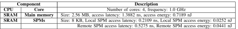
TABLE VI.
SYSTEM SPECIFICATION FOR SPM, L2 MEMORY AND MAIN MEMORY
Component Description
CPU Core Number of cores: 4, frequency: 1.0 GHz
SRAM Main memory Size: 2.56 MB, access latency: 1.3882 ns, access energy: 0.7189 nJ
SRAM SPMs Size: 8 KB, Local SPM access latency: 0.2109 ns, Local SPM access energy: 0.0252 nJ Remote SPM access latency: 0.5275 ns, Remote SPM access energy: 0.0441 nJ
the same size, with the capacity of 8 KB. We also assume the capacity of the off-chip main memory is 2.56 MB, which is large enough to store all data items. A set of parameters collected from CACTI tools provided by HP for these two memory types is shown in Table VI.
A custom simulator based on SimpleScalar is devel-oped to simulate the process of data distribution and obtain costs of memory accesses for the program. With the CACTI tools [23] provided by HP, we can obtain the latency and energy consumptions for memory accesses, then we use them as parameters on our benchmark pro-grams. In the experiment, we run random, greedy and the dynamic programming algorithm IOLDD. Compute the time cost and energy consumption for all data accesses. Our program is easy to compatibly integrate into any compiler.
B. Experimental Results
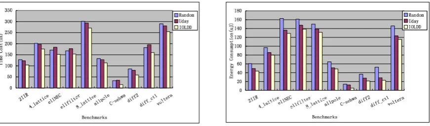
In Fig. 5, algorithms are compared via ten bench-marks include: 2IIR, 4-lattice, ellENC, ellfilter, 8-lattice, allpole, C-sehwa, diff2, diff-ct1 and voltera. Time costs and energy consumptions of data distributions on multi-core systems are also presented. In Tab. VII, the column “Random” represents the algorithm that data items are randomly picked and distributed to four on-chip SPMs of the cores. Due to the randomness of the technique, the experiment is precessed 10 times to get an aver-age number. The column “Uday” is a greedy algorithm proposed by the Udayakumaran’s algorithm [12]. The column “IOLDD” denotes our IOLDD algorithm. It is a dynamic programming algorithm applied into both array and scalar data items in loop on multi-core systems. The percentage of improvement for IOLDD algorithm over the “Random” technique is shown in column “Imprv (IOLDD/Random)”. The average improvement of time costs of the IOLDD algorithm is 18.45%. Moreover, “Imprv (IOLDD/Uday)” displays the improvement for “IOLDD” algorithm over “Uday” algorithm, and the average improvement is 18.38%. As shown in the exper-imental results, our IOLDD algorithm achieves the best improvement of time costs on average among all other techniques. In the best case, e.g. C-sehwa, the percentage of improvement in time cost is 52.12% over “Random” algorithm and 54.26% over “Uday” algorithm.
Not only data accesses time is reduced because of the effective solution of data distribution, but also the energy consumption lessens. Both Fig. 5 and Tab. VIII show the comparison of energy consumption among various data distribution solutions that are generated by various techniques. Accordingly, the average improvement of
IOLDD algorithm over random technique is 30.12%, and the average improvement of IOLDD algorithm over Uday algorithm is 14.52%, our IOLDD algorithm also achieves the best improvement of energy consumption. In the best case, e.g. C-sehwa, the percentage of improvement in energy consumption is 64.63% over “Random” algorithm and 57.99% over Uday algorithm.
Experiments indicate that IOLDD algorithm obtains better improvements in most of the time and energy costs compared with the Uday algorithm which employs a greedy strategy. The major advantages in techniques compared with the Uday algorithm can be seen in three parts. First, the IOLDD algorithm considers the initial data distribution of the loops and the effect of migrating data items. Therefore, it can generate the optimal solution for iterational data distribution. Second, the IOLDD algo-rithm takes the cost of updating array items into account and uses the relations of these array items to minimize the cost, while Uday algorithm does not. Third, the IOLDD algorithm uses the technique of duplication to reduce the cost.
VIII. CONCLUSION ANDFUTUREWORK
In this paper, we achieve the minimum cost of loop data distribution on multi-core systems by developing an Iterational Optimal Loop data Distribution algorithm with Duplication (IOLDD). The algorithm is used on multi-core systems, while the algorithm Zhanget al. proposed is limited to single-core systems and cannot fully utilize the benefits of the private SPM on each core [18]. The IOLDD algorithm improves the performance on multi-core sys-tems by taking the relations of an array, the updating cost and the duplication technique into consideration.
To explore more, in the future, we will further con-sider the problem of distributing loop data and avoiding contention when there are multiple “Write” activities on the same data for multiple cores. As to the mechanism of duplication, we will explore whether data still can be duplicated on condition that data is not read-only, and how to duplicate it. Besides, we will consider the problem when the main memory is a mixed structure of DRAM and non-volatile main memory (NVM). We will also deal with the problem of reducing the “Write” activities to the NVM in a heterogeneous system.
ACKNOWLEDGMENT
Figure 5. The corresponding time and energy results in the experiment.
TABLE VII.
COMPARISON OF TIME COSTS FOR VARIOUS DATA DISTRIBUTION ON MULTI-CORE SYSTEMS
Bench. Uday(µs) IOLDD(µs) Random(µs) imprv(IOLDD/Random) imprv(IOLDD/Uday)
2IIR 127.529 123.253 103.512 18.83% 16.02%
4-lattice 201.754 196.25 175.542 12.99% 10.55%
ellNEC 170.923 184.623 151.371 11.44% 18.01%
ellfilter 167.907 177.599 153.177 8.45% 13.45%
8-lattice 301.091 293.28 270.973 10.00% 7.61%
allpole 133.276 127.262 113.757 14.65% 10.61%
C-sehwa 33.708 35.276 16.135 52.12% 54.26%
diff2 86.786 80.113 59.106 31.89% 26.22%
diff-ct1 182.001 194.498 160.334 11.90% 17.57%
voltera 289.184 280.551 253.902 12.20% 9.50%
average 18.45% 18.38%
TABLE VIII.
COMPARISON OF ENERGY COSTS FOR VARIOUS DATA ALLOCATION ON MULTI-CORE SYSTEMS
Bench. Uday(µJ) IOLDD(µJ) Random(µJ) imprv(IOLDD/Random) imprv(IOLDD/Uday)
2IIR 60.907 49.595 43.800 28.09% 11.68%
4-lattice 96.981 85.855 79.562 17.96% 7.33%
ellNEC 162.593 136.499 129.285 20.49% 5.29%
ellfilter 160.928 147.844 138.316 14.05% 6.44%
8-lattice 150.268 138.562 131.525 12.47% 5.08%
allpole 64.624 50.679 131.525 12.47% 5.08%
C-sehwa 14.295 12.037 5.057 64.63% 57.99%
diff2 36.404 27.315 21.060 41.15% 22.90%
diff-ct1 52.201 28.084 23.122 55.71% 17.67%
voltera 145.837 123.716 115.588 20.74% 6.57%
average 30.12% 14.52%
REFERENCES
[1]
http://www.analog.com/static/imported-files/data sheets/ADSP-BF534 BF536 BF537.pdf, Analog Devices Inc., 2010.
[2] http://www-s.ti.com/cs/psheets/spns034c/spns034c.pdf, Texas Instruments Inc., 2012.
[3] http://www.nvidia.com/page/8800 tech briefs.html, nVIDIA Co., 2013.
[4] R. Banakar, S. Steinke, B.-S. Lee, M. Balakrishnan, and P. Marwedel, “Scratchpad memory: a design alternative for cache on-chip memory in embedded systems,” in
Hardware/Software Codesign, 2002. Proceedings of the Tenth International Symposium on, 2002, pp. 73–78. [5] L. Zhang, M. Qiu, W. Tseng, and E. Sha, “Variable
partitioning and scheduling for mpsoc with virtually shared scratch pad memory,” Journal of Signal Processing Sys-tems, vol. 58, no. 2, pp. 247–265, 2010.
[6] O. Avissar, R. Barua, and D. Stewart, “An optimal memory allocation scheme for scratch-pad-based embedded sys-tems,” ACM Trans. Embed. Comput. Syst., vol. 1, no. 1, pp. 6–26, Nov. 2002.
[7] P. R. Panda, N. D. Dutt, and A. Nicolau, “Efficient utilization of scratch-pad memory in embedded processor
applications,” in Proceedings of the 1997 European con-ference on Design and Test, ser. EDTC ’97, 1997. [8] P. Panda, D. Dutt, and A. Nicolau, “On-chip vs.
off-chip memory: the data partitioning problem in embedded processor-based systems,”ACM Trans. Des. Autom. Elec-tron. Syst., vol. 5, no. 3, pp. 682–704, Jul. 2000. [9] Y. Zhou, Q. Zhu, and Z. Y., “Spatial data dynamic
bal-ancing distribution method based on the minimum spatial proximity for parallel spatial database,” Journal of Soft-ware, vol. 6, no. 7, pp. 1337–1344, 2011.
[10] Q. Zhu and Y. Zhou, “Automatic connection of compo-nents for dynamic distributed applications,” Journal of Software, vol. 8, no. 6, pp. 1419–1427, 2011.
[11] Y. Xu, Z. Zhao, W. Wu, and Y. Zhao, “Rppa: A remote parallel program performance analysis tool,” Journal of Software, vol. 6, no. 12, pp. 2399–2406, 2011.
[12] S. Udayakumaran, A. Dominguez, and R. Barua, “Dy-namic allocation for scratch-pad memory using compile-time decisions,”ACM Trans. Embed. Comput. Syst., vol. 5, no. 2, pp. 472–511, May 2006.
conference on Compilers, architecture and synthesis for embedded systems, ser. In CASES ’03, 2003, pp. 276–286. [14] O. Ozturk, M. Kandemir, and I. Kolcu, “Shared scratch-pad memory space management,” in Quality Electronic Design, 2006. 7th International Symposium on, Mar. 2006, pp. 576–584.
[15] O. Ozturk, M. Kandemir, and S. Narayanan, “A scratch-pad memory aware dynamic loop scheduling algorithm,” inQuality Electronic Design, 2008. 9th International Sym-posium on, Mar. 2008, pp. 738–743.
[16] R. Thakur, A. Choudhary, and J. Ramanujam, “Efficient al-gorithms for array redistribution,”Parallel and Distributed Systems, IEEE Transactions on, vol. 7, no. 6, pp. 587–594, 1996.
[17] W. Huan, Z. Yang, M. Chen, and L. Ming, “Energy-oriented dynamic spm allocation based on time-slotted cache conflict graph,” inDesign, Automation Test in Eu-rope Conference Exhibition (DATE), 2010, 2010, pp. 598– 601.
[18] J. Zhang, T. Deng, Q. Gao, Q. Zhuge, and E.-M. Sha, “Optimizing data allocation for loops on embedded sys-tems with scratch-pad memory,” in Embedded and Real-Time Computing Systems and Applications (RTCSA), 2012 IEEE 18th International Conference on, aug. 2012, pp. 184 –191.
[19] Y. Guo, Q. Zhuge, J. Hu, M. Qiu, and E.-M. Sha, “Opti-mal data allocation for scratch-pad memory on embedded multi-core systems,” inParallel Processing (ICPP), 2011 International Conference on, Sep. 2011, pp. 464–471. [20] Y. Guo, Q. Zhuge, J. Hu, and E.-M. Sha, “Optimal
data placement for memory architectures with scratch-pad memories,” inTrust, Security and Privacy in Computing and Communications (TrustCom), 2011 IEEE 10th Inter-national Conference on, nov. 2011, pp. 1045 –1050. [21] O. Ozturk, M. Kandemir, G. Chen, M. Irwin, and
M. Karakoy, “Customized on-chip memories for embedded chip multiprocessors,” inDesign Automation Conference, 2005. Proceedings of the ASP-DAC 2005. Asia and South Pacific, vol. 2, 2005, pp. 743–748 Vol. 2.
[22] M. Kandemir, J. Ramanujam, and A. Choudhary, “Ex-ploiting shared scratch pad memory space in embedded multiprocessor systems,” inProceedings of the 39th annual Design Automation Conference. ACM, 2002, pp. 219– 224.
[23] “Cacti model.” http://www.hpl.hp.com/research/cacti/. Qiuyan Gao received her BSc in information security from Hunan University, China, in 2011. She is currently a Master Candidate at Hunan University of Communication Engineering, China. Her current research interest includes parallel architec-ture, embedded multi-core systems and optimization algorithms.
Qingfeng Zhuge received her Ph.D. from the Department of Computer Science at the University of Texas at Dallas in 2003. She obtained her BS and MS degrees in Electronics Engineering from Fudan University, Shanghai, China. She is now a full professor at Chongqing University, China.
She received Best Ph.D. Dissertation Award in 2003. She has published more than 60 research articles in premier journals and conferences. Her research interests include parallel architec-tures, embedded systems, supply-chain management, real-time systems, optimization algorithms, compilers and scheduling.
Jun Zhangreceived his BSc and MSc in computer science from Hunan University, China, in 2011 and 2013. He is currently a PhD candidate in Chongqing University, China. His research interests include high-performance computer and multi-core
embedded systems, real-time systems and information security.
Guanyu Zhuis currently a researcher and leader of storage and software group at Huawei Research Center. His research inter-ests include clustered storage architectures, design of memory architecture with non-volatile memory, storage management, and file systems.
Edwin Hsing-Mean Sha received Ph.D. degree from the De-partment of Computer Science, Princeton University, Princeton, NJ, in 1992. Since 2000, he has been a tenured full professor in the Department of Computer Science at the University of Texas at Dallas. Since 2012, he served as the Dean of College of Computer Science at Chongqing University, China. He has published more than 300 research papers in refereed conferences and journals. He has served as editors for many journals, and as program committee and Chairs for numerous international conferences.