Munich Personal RePEc Archive
Empirical policy functions as benchmarks
for evaluation of dynamic models
Bazdresch, Santiago and Kahn, R. Jay and Whited, Toni
University of Minnesota, University of Rochester, University of
Rochester
1 April 2011
Online at
https://mpra.ub.uni-muenchen.de/51568/
Empirical Policy Function Benchmarks for Evaluation
and Estimation of Dynamic Models
Santiago Bazdresch R. Jay Kahn Toni M. Whited∗
First Version: April 2011 This Version: November 2013
Empirical Policy Function Benchmarks for Evaluation and Estimation of Dynamic Models
Abstract
We describe a set of model-dependent statistical benchmarks that can be used to esti-mate and evaluate dynamic models of firms’ investment and financing. The benchmarks characterize the empirical counterparts of the models’ policy functions. These empirical policy functions (EPFs) are intuitively related to the corresponding model, their features can be estimated very easily and robustly, and they describe economically important as-pects of firms’ dynamic behavior. We calculate the benchmarks for a traditional trade-off model using Compustat data and use them to estimate some of its parameters. We present two Monte Carlo exercises, one that shows EPF-based estimation has lower average bias and lower variance than traditional moment-based estimation and another that shows EPF-based tests are better at detecting misspecification.
Keywords: trade-off model,structural models of capital structure, estimation of dynamic models, indirect inference, model evaluation
1
Introduction
A large literature in finance and economics studies dynamic models of the firm, in which
agents, period by period, optimally choose optimal decisions as a function of the current
state of their environment.1 While these sophisticated dynamic programming problems
are analytically complex and often only have approximate numerical solutions, this general
research endeavor is promising: investing and financing are intrinsically dynamic problems
that can only have a quantitatively satisfactory representation in a dynamic model.
More-over, dynamic models allow researchers to extract a wealth of time series and cross sectional
predictions with which to compare model and data. This richness allows researchers to
dis-cipline dynamic models more than static models. In general, this disdis-cipline is useful because
it allows the evaluation of different models’ ability to match the data, and ultimately, to
establish the quantitatively better theoretical bases for understanding firms’ behavior.
However, an issue of concern in the financing and investment literature is that there is
no agreement on the right predictions to use for disciplining these quantitative dynamic
models. Different researchers make different choices about which features of the data to
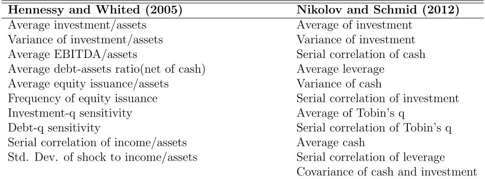
consider, as exemplified in Table 1, which lists two sets of benchmarks used in the literature.
The result is a wealth of different models, all of which claim that they successfully explain
the data, a situation that puts in question the scientific value of this type of research. A
methodology in which models are not falsifiable is not useful. This paper argues that,
instead of arbitrary features of the data, for each model there is a natural set of statistics
to be used for estimation and evaluation. Moreover, these statistics are, to a large extent,
common across existing specifications of investment and financing problems. Therefore,
they can be thought of as benchmarks that dynamic capital structure models should aim
1
to match. While we provide a number of these benchmarks for a particular capital structure
model, similar objects are easily calculated for any model. In this sense, we provide one
practical method to answer the typical “Which Moments to Match?” question of Gallant
and Tauchen (1996).
We derive these benchmarks from the model’s policy functions, which describe the
optimal response of the firm (the control variables) as a function of its environment (the
state variables). Our central argument is that the empirical counterpart of these policy
functions should be informative in the evaluation and estimation of a dynamic model.
Therefore, we develop a method for using robust estimates of the main features of these
empirical policy functions (EPFs) to estimating the parameters of dynamic models. Of
course, there are many ways to characterize an empirical relationship. In this paper, we
focus mainly on the first-order features of these EPFs, namely their slopes. Among these
features, we focus on statistically robust estimators, which insures that we are looking at
representative features of the data.
To estimate our EPFs we use only the within-firm variation of each of the relevant
variables. This practice is consistent with a typical model setup in which firms are ex-ante
homogeneous. The use of within-firm variation implies that we do not target the mean
values of any of the state or control variables. Instead, we use their variation across time
and states of nature. While it is possible that, for a particular model, there is a unique
feature of the data (such as the mean of a variable) that can help estimate its parameters,
our argument here is that a common set of benchmarks that captures the first order features
of the empirical policy functions should be a starting point with which to evaluate these
models.
Using EPFs as benchmarks for estimating and evaluating models confers several
benchmarks capture an economically important fraction of the variance of the control
vari-ables in the data. For example, out of the total dispersion of the investment to capital ratio
in the data, around 20% can be captured by the slope of the EPFs. Thus, our benchmarks
are describing a large fraction of what firms actually do.
Second, these benchmarks are intrinsically related to the economic dynamics of the
model. The point of writing dynamic models is that we have dynamic data to test them
against and therefore powerful tests of these models need to involve facts that describe
firms’ dynamics. In contrast to this principle, models in the literature are often estimated
or tested with respect to sample averages, such as mean leverage or mean cash holdings.
The third argument is that these quantities are often used already in some structural
estimations, so they are not large departures from tradition. Instead what we propose in
this paper is a transparent, simple, robust method for choosing and computing benchmarks
that can potentially let us compare one model to another meaningfully.
We conduct several Monte Carlo exercises to gauge the finite-sample performance of
estimators that use empirical EPFs, and we compare these estimators to ones that use
traditional moments. We find two important results. First, estimation with these EPF
benchmarks generates parameter estimates that are less variable and have less bias than
those generated with moments. Second, estimation with these EPF benchmarks leads to
specification tests that have more power to reject misspecified models.
Although our paper is clearly related to the many applied papers that have used
simu-lated method of moments to estimate the parameters of dynamic models, it is more closely
related to a set of papers that deal with estimation of dynamic oligopoly games in
indus-trial organization. For example, Rust (1994) describes a set of methods for solving and
Bajari, Benkard, and Levin (2007) describe two-step algorithms for estimating a dynamic
game under particular assumptions about the game’s equilibrium. The estimation method
proposed by Bajari et al. (2007) is closely related to the one in this paper and focuses on
estimating the policy functions as the essential quantities to input into a simulated
mini-mum distance estimator. Our paper stands apart from this literature because our methods
are “full-solution” methods that actually match theoretical and estimated policy functions.
This paper proceeds as follows: Section 2 of the paper presents a generic model and
detailed steps for benchmark calculation, a measure of the explanatory power of a model,
and a brief description of indirect inference and bootstrapping as applied here; section 3
presents a generic dynamic trade-off model of capital structure, along with its benchmarks,
and a comparison of indirect inference performed with traditional moments and with our
benchmarks; section 5 presents two Monte Carlo exercises, the first, a parameter recovery
experiment that shows our benchmarks generate parameter estimates with lower volatility
and bias, and the second that shows that our benchmarks are better at detecting
mis-specification; section 6 concludes.
2
Benchmarks and Estimation
2.1
Generic Model
The models of the firm that we consider can be described generically in terms of a Bellman
equation:
V(x) = max
h
n
D(x, h) +βE(V (x′)|x, h)o, (1)
in which x is an M = N +K vector of state variables, with a prime indicating tomorrow
can be directly manipulated by the N vector of control variables,h, as well asK exogenous
stochastic state variables, which follow a Markov process. The control and state variables
are linked via a law of motion given by
x′ ≡g(x, h) (2)
V(x) represents the market value of the firm’s equity, D(x, h) represents payments to
or from shareholders, β is the discount factor and E(· | x, h) is the expectation with
respect to the Markov transition function, given x and h. For example, the variable x
typically contains the firm’s capital, leverage, and a profitability shock. The vector of
control variables typically contains investment and debt issuance. The firm observes xand
then maximizes the present discounted value of the sum of current and future dividends by
setting the control variable h optimally during each period.
In this generic setup, the solution of the model consists of the optimal policy function
H(x) and the value function of the firm V(x). The policy and value functions satisfy the
following system:
H(x) = argmax
h
n
D(x, h) +βE(V (x′)|x, h)o (3)
and
V(x) = D(x, H(x)) +βE(V (x′)|x, H(x)) (4)
For simplicity, we assume that all of the state variables are observable. As we show below,
however, in many of the cases in which some of the stochastic state variables are
unobserv-able, the policy function can be expressed in terms of observable transformations of the
2.2
Benchmarks
Given the process for exogenous variables, the policy function H(x) characterizes the
solu-tion of the model. It is the main object that translates the assumpsolu-tions of the model into
a functional prediction about the firm’s actions in different situations. Therefore, a direct,
simple and theoretically motivated way to evaluate a dynamic model is to evaluate its
abil-ity to replicate the firms’ observed policies. In this paper we argue that a good approach
to doing this is to characterize firms’ policy functions empirically, and then use this
char-acterizations as the objectives in structural model estimation and evaluation. This section
describes one robust way to characterize the first-order and the second-order features of
these objects, i.e. their slope and convexity.
Empirical Policy Functions
In order to obtain empirical policy function estimates it is necessary to have estimates of
the state in which firms are and of the policies that they follow in each state. We use
a simple process, inspired in the portfolio formation frequently used in the asset pricing
literature, to summarize these objects in a few key numbers.
The empirically estimated equivalent of the function H(x) is an estimated function ˆH
such that:
ˆ
H(x) = Hˆ1(x),Hˆ2(x), . . . ,HˆN(x). (5)
where ˆHn(x) represents the average or the median behavior along control dimension n for
firms that observe a value x for the state variable. A typical procedure is to use regression
analysis to estimateHas a linear function of x, however that procedure is not robust to the
presence of outliers or to the possibility of nonlinearity. Therefore we characterize Hˆ(x)
estimating the median choice for the control variables for all firms within a particular bin
as described in detail below.
Step 1: Demean each state and control variable at the firm level. This step is important because the models described and exemplified above are typically models where firms are
ex-ante homogenous. Also, we are concerned mainly with the dynamics of the different
variables, as opposed to any cross-sectional variation. Label the demeaned state variables
as xi,t and control variables ashi,t for each firm-period observation.
Step 2: GenerateB equally spaced bins across each of the state variables of the model. For example, if we use five binds, we define the bins as the 0%–20%, 20%–40%, 40%–60%, 60%–
80% and 80%–100% percentiles of each state variable and label them from 1 to 5. Classify
each observation of each state variable as belonging into one variable-specific bin. This
classification is done independently for each variable, that is, it is non-sequential sorting.
Each firm-period observation is therefore given a classification as b(xi,t) = (b1, b2, . . . , bM),
with each bm representing state variable m’s bin classification for that firm in that period.
Similarly, classify the control variables in bins c(hi,t) = (c1, c2, . . . , cN).
Step 3: Estimate the policy function for control variable n as functions of state variable
m as the median observed choice within each of the (composite) bins:
ˆ
Hn
m(B) = median{i,t|bm(xi,t)=B}(h n
i,t). (6)
Step 4: Finally, characterize the features of Hˆ(x) by comparing the policies over bins across each state variable. Here, we consider both slope and curvature. The first-order
features (the slope) of the policy function can be characterized as the ratio of the difference
state variable in those bins:
βn
m(1, B) =
ˆ
Hn
m(B)−Hˆmn(1)
˜
x|bm(x)=B −x˜|bm(x)=1
, (7)
in which ˜x|bm(x)=krepresents the median value of the state variable xin thek
th bin of that
variable.
The second order features (the curvature) of the policy function can be characterized
as the ratio of the change in slope over the state variable to the range of that particular
state variable.
Γnm(1, B) =
βn
m(B/2, B)−βmn(1, B/2)
(˜x|bm(x)=B −x˜|bm(x)=1)/2
(8)
2.3
Potential Explanatory Power
An important question in evaluating a dynamic model of the firm is how much of the
actual behavior of the firm can we expect to rationalize. We define a robust measure of
this quantity as follows:
P Emn =
˜
hn
i,t |i,t|bm(xi,t)=B −h˜ n
i,t |i,t|bm(xi,t)=1
˜
hn
i,t |i,t|cn(h
i,t)=B −h˜ n
i,t |i,t|cn(h i,t)=1
(9)
where ˜hn
i,t |i,t|cn(h
i,t)=k represents the median of the n
th control variable in the kth quintile
of the empirical hm distribution and ˜hn
i,t |i,t|bm(xi,t)= k represents the median value of h n
for data observations where the mth state variable is in the kth quintile of the empirical x
m
distribution. A large value of this ratio suggests that a large fraction of the total variance
of the control variable hn in the data can potentially be explained by a model in which hn
2.4
Benchmark’s Variance-Covariance
The statistics described above are not traditional moments in the sense of being sample
averages of a function of each observation. Therefore, the standard methods to obtain
estimates of the variance and covariance of an estimate or vector of estimates are not
useful in this case. This section describes how we estimate the variance and covariance of
the statistics described above.2
2.5
Bootstrapping
One way to obtain a measure of the variance of the estimators described above is through
bootstrapping. The bootstrapping procedure uses the variation of the estimator across
different artificial samples as a measure of the volatility of the estimator. These artificial
samples are drawn from the original sample and used to recalculate the estimator. The
estimation is then performed for a J bootstrapped samples. The variation of the estimator
in the population is then estimated to be similar to the variation across the different
estimates obtained in this way.
We perform bootstrapping on our estimators by sampling with replacement, taking the
time series of each firm as one element of the sample. The estimate of the variance of an
estimator ˆθ is
ˆ
V(θ) = (1/J)
J
X
j=1
θsj −θ¯ˆ)′(θsj −θ¯ˆ
(10)
where is θsj is the estimator evaluated with the sample sj and ˆθ is the mean over j ∈
{1, . . . , J} of θsj.
2
2.6
Indirect Inference
Once the above benchmarks are calculated we can use them to estimate a model through
the indirect inference procedure in Smith (1993) and Gourieroux, Monfort, and Renault
(1993).We now briefly describe the procedure, as it applies to our policy function
bench-marks. First, we now explicitly allow the policy and value functions, h = H(x, θ) and
V(x, θ), to depend on a vector of structural model parameters, θ. These parameters
in-clude such quantities as the curvature of a production function, the variance of an exogenous
state variable, or a cost of external finance. On an intuitive level, it might be desirable
to estimate θ via maximum likelihood. However, for most dynamic models of the firm, a
closed-form likelihood is not available. Indirect inference fills this gap by using an
auxil-iary model, with its own parameter vector, b. This auxiliary model should ideally capture
important features of the data. The goal is then to estimate θ by minimizing the distance
between the parameter vector of the auxiliary model, b, estimated with a real data set and
the same parameter parameter vector estimated with data simulated from a model.
Let yT be a real data matrix of lengthT, Without loss of generality, the parameters of
the auxiliary model can be represented as the solution to the maximization of a criterion
function
bT = argmax b
JT (yT, b),
The simulation of data from the model in section 2.1 proceeds as follows. First, givenθ,
pick a starting value for x,x0. Next, updatex0 by by using the policy function to generate
h, and then using the law of motion to generate x′, and so on. Let ys
t be the resulting
simulated data matrix of length T from simulation s, s= 1, . . . , S. For each of these data
bs
T (b) = arg maxb JT (xsT, b s(b)),
Note that the bs
T(b), as explicit functions of the structural parameters, θ.
The indirect estimator of b is then defined as the solution to the minimization of
ˆ
θ = arg min
b
"
bT −
1
S
S
X
h=1
bsT (θ)
#′
ˆ
WT
"
bT −
1
S
S
X
h=1
bsT(θ)
#
(11)
≡ arg min
b
ˆ
G′TWˆTGˆT, (12)
in which ˆWT is a positive definite matrix that converges in probability to a deterministic
positive definite matrix W. We use the the optimal weight matrix, which is the inverse of
the covariance matrix of θ described in Section 2.5.
The indirect estimator is asymptotically normal for fixedS. Define J ≡plimT→∞(JT).
Then
√
Nθˆ−θ−→ Nd 0,avar(ˆθ)
where
avar(ˆθ)≡
1 + 1
S " ∂J ∂b∂θ′ ∂J ∂b ∂J′ ∂b −1 ∂J ∂θ∂b′
#−1
.
The technique provides a test of the overidentifying restrictions of the model, with
T S
1 +SGˆ
′
TWˆTGˆT
converging in distribution to a χ2, with degrees of freedom equal to the dimension of θ
minus the dimension of b.
3
Trade-Off Model
In this section we show the results of an indirect inference structural estimation using
from a trade-off model and then perform indirect inference on data simulated by that
model. We then describe the ability of the two indirect inference procedures to recover the
parameters of the original model. We compare the two estimations in terms of average bias
and estimator volatility. The rest of this section describes an example of a model in this
literature. It is a simplified version of Hennessy and Whited (2005):
The firm’s cash flow
We consider a firm that uses capital, Kt to generate operating income according toAtKtα,
where Kt is capital, 0 < α < 1 is a parameter that governs returns to scale, and At is a
productivity shock. The productivity shock, At, is lognormally distributed and follows the
process given by:
ln(At) = ¯A+ρln(At−1) +σεt, εt ∼ N(0,1) (13)
The firm’s cash flow (Et) is its operating income plus its net debt issuance ∆Bt, minus
its net expenditure on investment, C(It), and minus its interest payments on debt,BtrBt :
Et =AtKtα−C(It) + ∆Bt−BtrBt (Bt, Kt) (14)
In 14, It is defined by a standard capital stock accounting identity:
Kt+1 ≡Kt(1−δ) +It (15)
Similarly, net debt issuance, ∆Bt is defined by
Bt+1 ≡Bt+ ∆Bt (16)
Dividends and equity issuance
The firm’s dividends and equity issuance are defined in terms of the firm’s cash flows. A
stockholders, a negative cash flow implies that the firm’s optimal decision is to set dividends
at 0 and instead obtain funds from the equity market (Xt=−Et).
Et >0 ⇒ Dt=Et, Xt = 0 (17)
Et≤0 ⇒ Dt= 0, Xt= (1 +λ)(−Et), (18)
in which λ stands for the proportional cost of issuing equity.
Real sector frictions
The firm faces a set of frictions. Consistent with most of the literature it faces convex
costs of investment as well as some degree of investment irreversibility. The firm’s cost
of investment function includes the cost of purchasing the capital, plus a convex cost of
investment and plus an investment irreversibility term.
C(It) =It+γKt(It/Kt)2−ξKtI(It<0), (19)
whereγrepresents the magnitude of convex costs of investment, ξrepresents the magnitude
of fixed costs of investment, andI(It>0) represents an identifier function that is 1 ifIt>0
and 0 otherwise.
Interest rate on debt
The interest rate on debt is a risk free rate plus a ‘risk premium’, an increasing, convex
function of leverage:
rB
The firm’s optimization problem
The firms problem is to maximize the discounted value of dividends for current owners
of the firm. With this objective the firm chooses investment and net debt issuance. The
resulting Bellman equation is then given by:
V(Kt, Bt, At) = max It,∆Bt
n
DtIEt>0+ (1 +λ)XtIEt<0+EtV(Kt+1, Bt1, At+1),
o
, (21)
subject to (15) and (16). Here, I is an indicator function.
State space and control space transformations
In the model above, Kt, At and Bt are the state variables and It and ∆Bt are the control
variables. However, At is an unobservable shock. Therefore, to estimate the parameters
of this model, we need to work with observable transformations of the state and control
variables. Further, because thelevelsof therealKtandBtare only defined up to a constant
of proportionality defined by an arbitrary price index. We therefore work with variables in
ratio form. We use the investment rate It/Kt and the debt issuance rate ∆Bt/Kt as the
control variables of the model. Similarly, we use profitability, Πt ≡AtKtα/Kt, and leverage,
Lt =Bt/Kt, as the state variables of the model.3
4
Benchmarks for Trade-Off Model
4.1
Data
We draw our sample of firms from the Compustat database from 1962 to 2012. We screen
the sample as follows. The firm must have a CRSP share code of 10 or 11. We then
drop all firms with fewer than two years of data, or that belong to the financial (SIC
code 6) or regulated (SIC code 49) sectors. Finally, we observations in which any of the
3
Note that, as in most capital structure and investment models, once At or Πt as defined above are
variables we use are missing. We define the following variables to be used in the rest of the
analysis. Book Leverage is (DLC +DLTT)/AT, Profitability is OIBDP/GPPE, Investment
is CAPX/GPPE, and Debt Issuance is ∆ (DLC + DLTT)/AT.
4.2
Summary Statistics
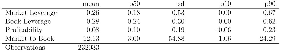
Table 2 presents the summary statistics of the state and control variables of the model as
defined above. Note that the values are consistent with other similar studies. The zero
value for the 10th percentile of investment rates and the 50th percentile of debt issuance
is consistent with research on lumpiness in the investment and financing literature.
The variation of the state variables is an essential quantitative feature of the data. As
the summary statistics show, the bottom quintile of profitability is about 16% lower than
the mean, while the top quintile is about 13% higher, so that the 5–1 inter-quintile range is
about 29% of average profitability. With respect to leverage it shows that the inter-quintile
range is about 62% of total assets, evenly distributed above and below the mean.
4.3
First-Order Benchmarks
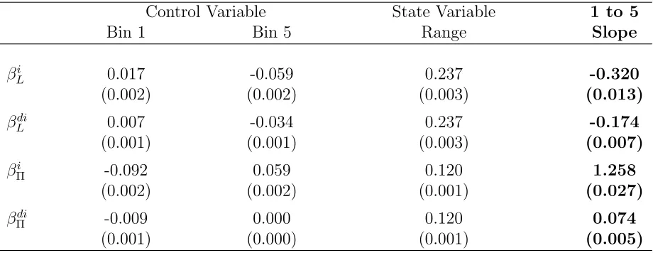
Table 3 describes the estimates of the first-order features (i.e the slopes) of the firm’s
policy functions. It shows the result of grouping each firm year observation according to
the value of productivity and leverage into quintiles and then obtaining the median policy
of firms in these bins in terms of investment and debt issuance. The main results are the
policy function slopes in the last column of the table. It shows that each percentage point
of leverage reduces investment by 0.32 percentage points, and reduces debt issuance by
0.17 percentage points. Also, it shows that each percentage point of profitability increases
investment by 1.26 percentage points and increases debt issuance by 0.07 percentage points.
precision, with all of the standard errors lying below 10% of the estimated value.
4.4
Second-Order Benchmarks
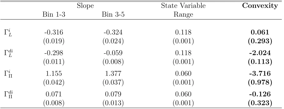
Table 4 describes the estimates of the second order features in the data. It shows that
investment is concave in leverage, that is, investment is more affected by debt at high
leverage levels. In contrast, debt issuance policy is convex in leverage, that is, it is less
sensitive to leverage at high leverage levels. Also, investment convex in profitability, that
is, it is more sensitive to profitability at high profitability levels. Finally, it shows that
the slopes of debt increase relative to profitability are not significantly different at high
and low profitability levels. Note that for brevity, we do not use these benchmarks in the
estimation exercises that follow.
4.5
Covariance Matrix of the Policy Function Benchmarks
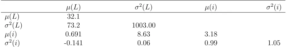
The indirect inference procedure requires, ideally, that one use the inverse of the
variance-covariance matrix of the policy function slopes, ˆWT, to normalize the distance between
the real-data and simulated policy function slopes. As described in section 2.4 above,
one way to estimate this matrix is through bootstrapping, which is what we do in this
paper. Below we compare the performance of a traditional moments-based estimation with
an estimation based on our policy function benchmarks. As a first step, Tables 6 and 7
describe the bootstrap-estimated variance-covariance matrices for both the moments and
policy functions we use. The main feature of this table is that the traditional moments
are substantially less variable than the EPF benchmarks. This result makes sense in that
4.6
Estimation Results
Table 8 describes the results of using the two different sets of empirical benchmarks to
estimate the parameters of the Trade-Off model. It shows that the results are substantially
different depending on the benchmark used. The EPF-based benchmarks result in a higher
estimate of capital adjustment costs, a lower estimate of the credit risk growth coefficient
and of the fixed cost of investment. The minimum value of the distance function is much
larger in the case of the EPF model. We interpret this difference as implying that the
EPF-based benchmarks are more powerful at detecting model misspecification.
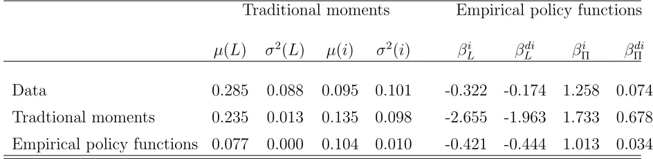
Table 9 displays the results of the indirect inference estimation of the trade-off model
from the point of view of the value of the different benchmarks with each of the two
estimated sets of parameters. It shows that, as expected, the EPF-based inference generates
a model whose benchmarks are closer to the EPF-benchmarks in the data, and vice versa,
the TM-based inference generates a model whose benchmarks that are closer to the TM
benchmarks in the data.
Moreover, this table lets us highlight one of the key advantages of focusing on EPF-based
benchmarks. The advantage is that the the distance between the EPF-based benchmarks
in the data and in the estimated model have a clear, useful interpretation, in contrast to the
same distance between TM-benchmarks. Comparing the first and third row of the second
set of columns of the table shows that in the estimated Trade-Off model a unit of leverage
increase leads to 0.421 units decrease in the investment rate, compared to 0.321 in the
data, a unit of leverage decreases debt issuance by 0.444 units, compared to 0.174 in the
data, a unit of profitability increases investment by 1.013 units compared to 1.258 in the
data and a unit of profitability increases debt issuance by 0.034 compared to 0.074 in the
too sensitive to leverage, and not sensitive enough to profitability. These conclusions are a
useful way to contrast the model with the data from the point of view of capital structure
theory.
Finally, comparing the first and second lines of this table suggest that although the
Indirect Inference estimation of the Trade-Off model with TM-based benchmarks is able
to generate TM-benchmarks that are close in the data and in the model, the estimated
model is not able to replicate the main quantitative relationships between variables in the
model. Investment and debt issuance are an order of magnitude too sensitive to leverage
and debt issuance is an order of magnitude to sensitive to profitability. While the
EPF-basd estimation leads TM-based benchmarks that are also very much off the mark, it is
not clear how to interpret these distances meaningfully.
4.7
Potential Explanatory Power of the Trade-Off Model
Relative Variation: State and Control Variables
An essential measure of whether our theories explain the data is one that compares the
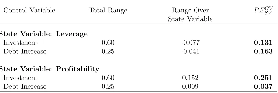
relative variation of explanatory and dependent variables. The figures in table 5 show this
comparison. These are one set of benchmarks for dynamic model evaluation: they describe
the relative variation in the data between state variables and control variables. Under this
measure a quantitatively good dynamic model of investment and debt issuance that as a
function of changing profitability and current leverage is one that replicates the relative
variation in investment and debt issuance with respect to leverage and profitability.
Table 5 describes this relative variation. It shows that the variation range of investment
along the leverage state variable is 13.1% of the total variation range of investment.
Simi-larly the variation of debt issuance along the leverage state variable is equivalent to 16.3%
for investment and 3.7% for debt issuance. These figures provide a measure of how much
of the variation in each of these variables we could expect a dynamic model with leverage
and profitability as state variables to explain.
5
Monte Carlo Exercises
This section describes the results of a set of Monte Carlo experiments that put to test
the intuition described above. These results are important in the sense that they show
that in a practical sense, estimation using EPF-based benchmarks produces better results
than estimation using traditional moments. We design these experiments as follows. Each
Monte Carlo is based on 100 simulated data sets. Each data set has a length of 50 and
a cross-sectional size of 3,000. These dimensions are roughly the average time-series and
cross-sectional dimensions of our real data set. We create our simulated samples as follows.
First, we choose values for three key parameters: the variable and fixed costs of adjustment
of the capital stock, γ = 1 and ξ= 0.03, and the premium on debt financing,Rrp = 2. To
keep the Monte Carlo tractable, we treat the curvature of the profit function, α, and the
parameters that govern the process for AT, σ and ρ, as known, setting them to 0.8, 0.15,
and 0.65, respectively.
5.1
Parameter Recovery
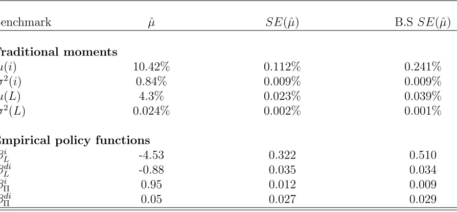
Table 10 describes the mean and the variance of two sets of statistics that can be used to
estimate a structural model. The first one is a set of traditional moments. The second
set corresponds to the slopes of the empirical policy functions as described above. The
statistics come from simulated data from the model above. The first column of the table
shows the simulated means of the different benchmarks. The second and third columns
ways. The first calculation is simply the standard deviation across the different Monte
Carlo trials. The second measure comes from simulating the model once and then taking
bootstrapping the benchmark by sampling with replacement over the firms in the sample.
This exercise suggests that, in this example, bootstrapping provides very good estimates
of the variance of the benchmark, which gives us confidence in the bootstrap estimates of
the empirical variance covariance matrices given before.
Table 10 describes a set of empirical estimates that we use for structural estimation. It
consists of two panels, each describing the means and two estimates of the standard error of
that mean. The first standard error estimate, in column 2, consists of the error calculated as
the standard deviation of the mean observed for different repetitions of model simulations.
The second estimate, in column 2, uses bootstrapping calculating a set of means through
sampling from individual firms in the first simulation. The table shows that, in the model,
the firm level bootstrapping estimate of the standard error of the mean provides a good
approximation to standard deviation of the estimate across different simulations.
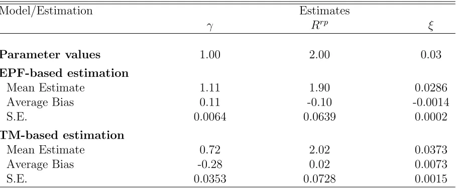
Table 11 shows the results of a Monte Carlo experiment estimating the trade-off model
described above using both the traditional moment-based and EPF benchmarks for
estima-tion. Both methods are able to get close to the parameter values of the model. However,
the estimation where direct inference uses EPF-type statistics performs better than the one
where the same procedure uses traditional moment statistics. The EPF based estimation
results in significantly lower bias in two out of three parameters, but most importantly in
dramatically reduced variance of the estimators. The variance reduction is of the order of
5.2
Power of Specification Tests
The last comparison we perform between estimation with traditional moments and
estima-tion with EPF-based moments focuses on mis-specificaestima-tion tests. An important concern in
economics is our ability to tell whether a model fits the data well enough or not. One such
test is a misspecification test. In the case of indirect inference, an available test is obtained
by a comparison of the distance between the estimated parameters of the auxiliary model
in the data and in the model with its theoretical distribution. Under conditions specified in
Gourieroux et al. (1993) the objective function described in equation 11 has a well defined
Ξ2 distribution.
In order to asses the power of different benchmarks to detect mis-specification we
per-form a Monte Carlo experiment. The experiment consists of simulating data from a know
model and then using simulated data from this known model to estimate the parameters
of two models: a well specified model and a misspecified model. We perform both of
these estimations twice, first using traditional moments as benchmarks and second with
the EPF-based benchmarks. We then compare the rejection power of tests based on each
one.
The misspecified model is similar to the one in section 3, but where the smooth risk
premium function has been substituted with a collateral constraint. In other words, the
interest rate equation, 20 in section 3, has been substituted for
rBt =R rf
IBt < λKt+RrfIBt>=µKt
i.e. a flat interest equal to the risk free rate as long as book leverage is below µ and a
100% interest rate otherwise. In the mis-specified model estimation, we estimate µinstead
Table 12 presents the results of the exercise described above. It shows that while
indirect inference of a well-specified model yields similar values for the objective function
for both the TM and EPF benchmarks, this is not the case for a mis-specified model. We
interpret this result as implying that the EPF benchmarks are (much) better at detecting
mis-specification without rejecting the true model more often.
6
Conclusion
We describe a set of benchmarks that we use for the quantitative evaluation of dynamic
corporate finance models. The benchmarks are a small set of numbers that characterize
the empirical counterparts of the policy functions from these models, which provide the
optimal firm policies, given the current state of the firm. We then describe a simple set
of steps to calculate these EPF-based benchmarks. We argue that these benchmarks are
intuitive, robust and theoretically motivated.
We then calculate these benchmarks for a typical dynamic capital structure model, and
use them to estimate the model. We also estimate the model using traditional moments.
We confirm that, in the estimation of the model, the choice of benchmarks is important.
Different benchmarks generate different parameter estimates when using them for indirect
inference.
We then show in first a Monte Carlo exercise that estimation with the proposed
bench-marks results in less biased and less variable estimates of the parameters of the model,
relative to a standard moments-based estimation. In a second Monte Carlo exercise, we
show that a specification test based on our proposed benchmarks has more power than the
same test based on traditional moments. It rejects the misspecified model more often, even
References
Aguirregabiria, Victor, and Pedro Mira, 2007, Sequential estimation of dynamic discrete games, Econometrica 75, 1–53.
Bajari, Patrick, C. Lanier Benkard, and Jonathan Levin, 2007, Estimating dynamic models of imperfect competition, Econometrica 75, 1331–1370.
Eckstein, Zvi, and Kenneth I. Wolpin, 1989, The specification and estimation of dynamic stochastic discrete choice models: A survey, The Journal of Human Resources 24, pp. 562–598.
Gallant, A. Ronald, and George Tauchen, 1996, Which moments to match?, Econometric Theory 12, 657–681.
Gourieroux, Christian S., Alain Monfort, and Eric Renault, 1993, Indirect inference, Jour-nal of Applied Econometrics 8, S85–S118.
Hennessy, Christopher A., and Toni M. Whited, 2005, Debt dynamics, Journal of Finance 60, 1129–1165.
Nikolov, Boris, and Lukas Schmid, 2012, Testing dynamic agency theory via structural estimation, Manuscript, University of Rochester.
Rust, John, 1994, Structural estimation of Markov decision processes, in R. F. Engle, and D. McFadden, eds., Handbook of Econometrics, volume 4, chapter 51, 3081–3143 (Elsevier).
Smith, Anthony A., Jr., 1993, Estimating nonlinear time-series models using simulated vector autoregressions, Journal of Applied Econometrics 8, 63–84.
Table 1: Examples of matching statistics used in the capital structure literature
Hennessy and Whited (2005) Nikolov and Schmid (2012)
Average investment/assets Average of investment Variance of investment/assets Variance of investment Average EBITDA/assets Serial correlation of cash Average debt-assets ratio(net of cash) Average leverage
Average equity issuance/assets Variance of cash
Frequency of equity issuance Serial correlation of investment Investment-q sensitivity Average of Tobin’s q
Debt-q sensitivity Serial correlation of Tobin’s q Serial correlation of income/assets Average cash
Std. Dev. of shock to income/assets Serial correlation of leverage Covariance of cash and investment
Table 2: Summary Statistics: State Variables
mean p50 sd p10 p90
Market Leverage 0.26 0.18 0.53 0.00 0.67
Book Leverage 0.28 0.24 0.30 0.00 0.62
Profitability 0.08 0.10 0.19 −0.06 0.23
Market to Book 12.13 3.60 54.88 1.06 24.29
Observations 232033
Table 3: Empirical Policy Function Slopes
Control Variable State Variable 1 to 5
Bin 1 Bin 5 Range Slope
βi
L 0.017 -0.059 0.237 -0.320
(0.002) (0.002) (0.003) (0.013)
βdi
L 0.007 -0.034 0.237 -0.174
(0.001) (0.001) (0.003) (0.007)
βi
Π -0.092 0.059 0.120 1.258
(0.002) (0.002) (0.001) (0.027)
βdi
Π -0.009 0.000 0.120 0.074
(0.001) (0.000) (0.001) (0.005)
Columns 1 and 2 describe the median of the policy function observations at time t for those firms classified in the first and 5th quintile of the state variable at time t−1. Columns 3 and 4 describe the median of the state variable at time t−1 in the 1st and 5th quintile bins for that variable. Column 5 describes the slope of the policy function calculated as (Control Bin 5- Control Bin 1)/(State Bin 1 - State Bin 5). Standard errors are calculated with bootstrapping, by sampling at the firm level. βi
L = slope of investmtent policy over leverage
state, βdi
L = slope of debt increase policy over leverage state,βΠi = slope of investment policy
over profitability state, and βdi
Π = slope of debt increase policy over profitability state. Data
Table 4: Table of Empirical Policy Function Convexities
Slope State Variable Convexity
Bin 1-3 Bin 3-5 Range
Γi
L -0.316 -0.324 0.118 0.061
(0.019) (0.024) (0.001) (0.293)
Γdi
L -0.298 -0.059 0.118 -2.024
(0.011) (0.008) (0.001) (0.113)
Γi
Π 1.155 1.377 0.060 -3.716
(0.042) (0.037) (0.001) (0.978)
Γdi
Π 0.071 0.079 0.060 -0.126
(0.008) (0.013) (0.001) (0.323)
Columns 1 and 2 describe the slope of the policy function approximated from the medians in the state variable quintiles 1 to 3 and 3 to 5. Columns 3 describes the corresponding range for the state variable. Column 4 describes the convexity of the policy function calculated as (Slope 3-5- Slope 1-3)/(State Var. Range). Standard errors are calculated with bootstrap-ping, by sampling at the firm level. Γi
L = convexity of investmtent policy over leverage state,
Γdi
L = convexity of debt increase policy over leverage state, ΓiΠ = convexity of investment
policy over profitability state, and Γdi
Π = convexity of debt increase policy over profitability
Table 5: Range of Control Variable Variation in the Data
Control Variable Total Range Range Over P ECV SV
State Variable
State Variable: Leverage
Investment 0.60 -0.077 0.131
Debt Increase 0.25 -0.041 0.163
State Variable: Profitability
Investment 0.60 0.152 0.251
Debt Increase 0.25 0.009 0.037
Table 6: Variance-Covariance Matrix, Traditional Moments
µ(L) σ2(L) µ(i) σ2(i)
µ(L) 32.1
σ2(L) 73.2 1003.00
µ(i) 0.691 8.63 3.18
σ2(i) -0.141 0.06 0.99 1.05
[image:32.612.72.542.487.566.2]Figures describe the variance-covariance matrix of the vector of statistics listed in the first column, estimated using bootstrapping over firms in the sample. All variables are multiplied by 10 million. Data is from Compustat. Variable definitions are in the appendix.
Table 7: Variance-Covariance Matrix, EFP based benchmarks
βi
L βLdi βΠi βΠi
βi
L 106
βdi
L 56.9 459
βi
Π -7.67 -20.3 639
βdi
Π 6.69 41.1 127 205
Table 8: Structural Estimates of Trade-Off model Parameters with Different Benchmarks
Benchmark type Estimated Parameters Minimum of
γ Rrp ξ Objective
Traditional moments -0.028 0.0525 0.046 16859.2 Empirical policy functions 1.031 0.658 0.035 28281.3
Coefficients obtained through indirect inference on the three parameters, Adjustment Costs, Credit Risk and Fixed Costs. Indirect inference performed by minimizing the (inverse co-variance matrix weighted) distance of the simulated values of each set of benchmarks from the corresponding values found in Compustat. γ is the cost of capital adjustment parame-ter, Rrp is the size parameter for the risk premium function, and ξ is the parameter of the
non-convex costs of capital adjustment.
Table 9: Benchmark Values at Indirect Inference Estimates, Trade-Off Model
Traditional moments Empirical policy functions
µ(L) σ2(L) µ(i) σ2(i) βi
L βLdi βΠi βΠdi
Data 0.285 0.088 0.095 0.101 -0.322 -0.174 1.258 0.074 Tradtional moments 0.235 0.013 0.135 0.098 -2.655 -1.963 1.733 0.678 Empirical policy functions 0.077 0.000 0.104 0.010 -0.421 -0.444 1.013 0.034
[image:33.612.73.545.459.574.2]Table 10: Measures of the Standard Error of Benchmarks, Simulated Data
Benchmark µˆ SE(ˆµ) B.S SE(ˆµ)
Traditional moments
µ(i) 10.42% 0.112% 0.241%
σ2(i) 0.84% 0.009% 0.009%
µ(L) 4.3% 0.023% 0.039%
σ2(L) 0.024% 0.002% 0.001%
Empirical policy functions
βi
L -4.53 0.322 0.510
βdi
L -0.88 0.035 0.034
βi
Π 0.95 0.012 0.009
βdi
Π 0.05 0.027 0.029
This table describes different measures of estimate standard errors. The means, sample volatility estimate, and bootstrapping estimate over repetitions are calculated with 30 rep-etitions of the model simulation. The bootstrapping within one repetition estimate is cal-culated by bootstrapping across firms in a single repetition of the simulation. i stands for the investment rate I/K, , distands for debt issuance rate DI/K, Π stands for profitability
AKα−1, and L stands for leverage.µ(·) stands for the mean, σ2(·) stands for the variance
and βn
m stands for the first order characterization of the policy for control variable n as a
Table 11: Comparison of Model Estimation with Different Matching Objectives
Model/Estimation Estimates
γ Rrp ξ
Parameter values 1.00 2.00 0.03
EPF-based estimation
Mean Estimate 1.11 1.90 0.0286
Average Bias 0.11 -0.10 -0.0014
S.E. 0.0064 0.0639 0.0002
TM-based estimation
Mean Estimate 0.72 2.02 0.0373
Average Bias -0.28 0.02 0.0073
S.E. 0.0353 0.0728 0.0015
Monte Carlo mean and standard error of Indirect Inference parameter estimates obtained with two sets of benchmarks, and corresponding model parameters.
Table 12: Comparison of Mis-specification Detection Power
Estimation Objective Function
Correct Model, TM-based estimation 15.5 Correct Model, EPF-based estimation 11.9 Mis-specified Model, TM-based estimation 233.8 Mis-specified Model, EPF-based estimation 1274.5